A Discrete Model of Three Species Prey- Predator System

Abstract

This paper investigates an eco-system with two prey species and a predator. The model equations constitute a set of three first order non-linear coupled difference equations. All possible positive equilibrium points of the model are computed and criteria for the stability of all equilibrium states are established. Simulations are performed in order to illustrate the theoretical results and gain further insight into the behaviour of the system

Keywords

predator-prey interactions, difference equations, equilibria, stability.

INTRODUCTION

Ecosystems are characterized by the interaction between different species and natural environment. Some important ecological interactions are Competition, Mutualism and Predation. The Lotka - Volterra predator prey equations were discovered independently by Alfred Lotka and by Vito Volterra in 1925-26. In 1926, Volterra devised a model to describe the evolution of predator and prey fish populations in the Adriatic Sea after the First World War (when fishing was curtailed). Population ecology typically focuses on particular species or pairs of species within webs of interacting species to understand variations in their abundance. Several papers appeared on 2-D models of predator - prey dynamics. Since the analysis of non linear systems when n > 2 (number of species) is much more difficult, only a limited amount of work is available on ‘Three Species Models’ [7,8].

II. RELATED WORK

There exists a vast amount of literature on prey predator models, see [3,5]. The classical Lotka - Volterra predator prey equations predicted neutral cycles with a period determined by parameters and amplitude set by initial conditions. Later, many authors studied the effect of prey predator interactions by introducing logistic growth expression, functional responses and Allee effect [2]. It was demonstrated that some of the simplest nonlinear difference equations describing the growth of biological populations with nonoverlapping generations can exhibit a remarkable complex and rich dynamical behaviour involving stability, existence of limit cycles, bifurcation and chaos [1,2,4,8,9]. In this paper, we investigate the stability nature of equilibria of a system describing the interaction among three species using a discrete model.

III. MODEL EQUATIONS

We are concerned with the following set of first order linear difference equations which models the interaction between two preys and one predator.

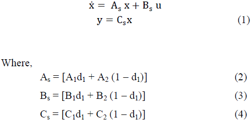where the parameters a, b, c, d and e are non-negative. The population of preys (x(n), y(n)) follow logistic growth model. The rate of predation is proportional to the rate at which the predator and the preys meet. This system of equations cannot be solved analytically, but some information about the behaviour of its solutions can be obtained via qualitative analysis. The mathematical analysis of the model is often used for the assessment of stability of the equilibrium.

IV. EXISTENCE OF EQUILIBRIUM OF THE SYSTEM AND A LEMMA

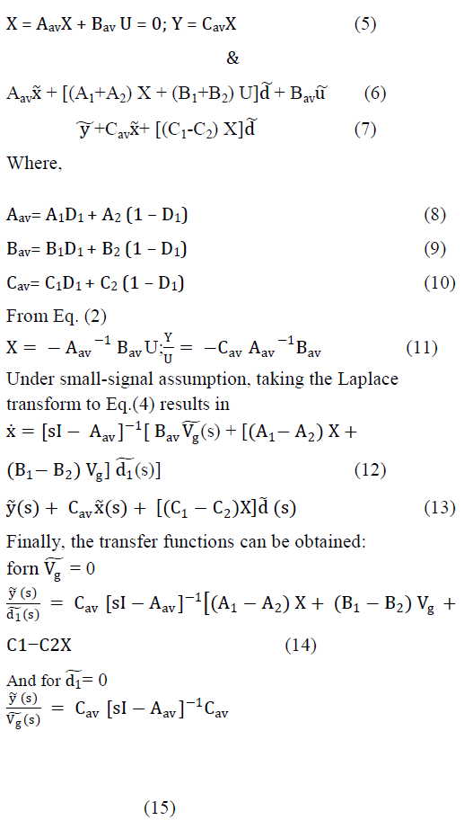The first equilibrium point E0 corresponds to the extinction of species in the eco-system where as E1 and E2 are axial equilibrium points corresponding to the situation in which two species become extinct. The equilibrium points E3, E4 and E5 correspond to the extinction of a species. The equilibrium points E6 is an interior equilibrium point which establishes the coexistence of all species in the system. The following Lemma is useful in the discussion of the stability properties of the equilibrium points of (1)

Lemma 1. Let [which can be found in (3)]

be the characteristic equation for a matrix. Then we have:

• If every root of equation (2) has absolute value less than one, then the equilibrium point of the system (1) is locally asymptotically stable and equilibrium point is called a sink.

V. STABILITY OF EQUILIBRIUM POINTS AND NUMERICAL STUDY

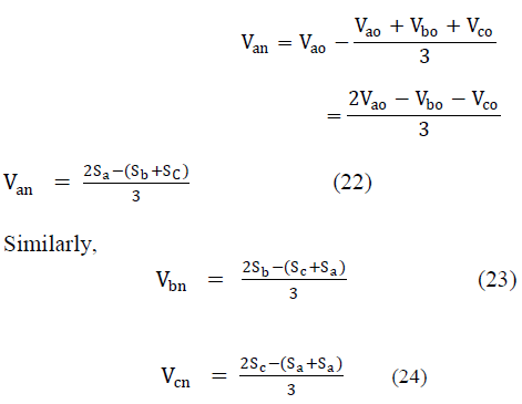
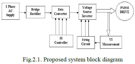
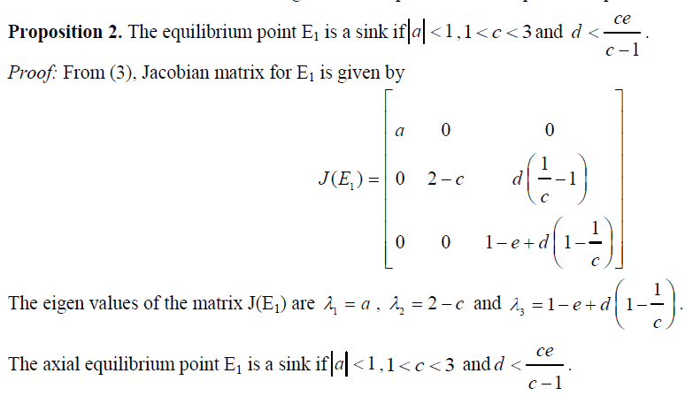
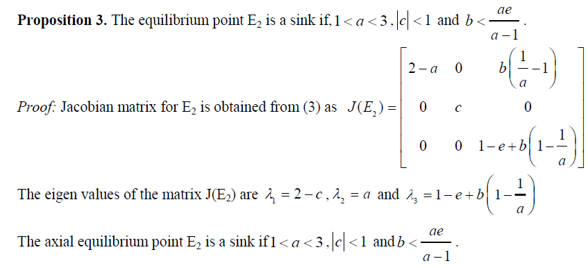
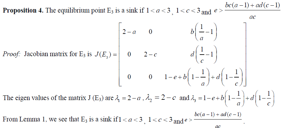
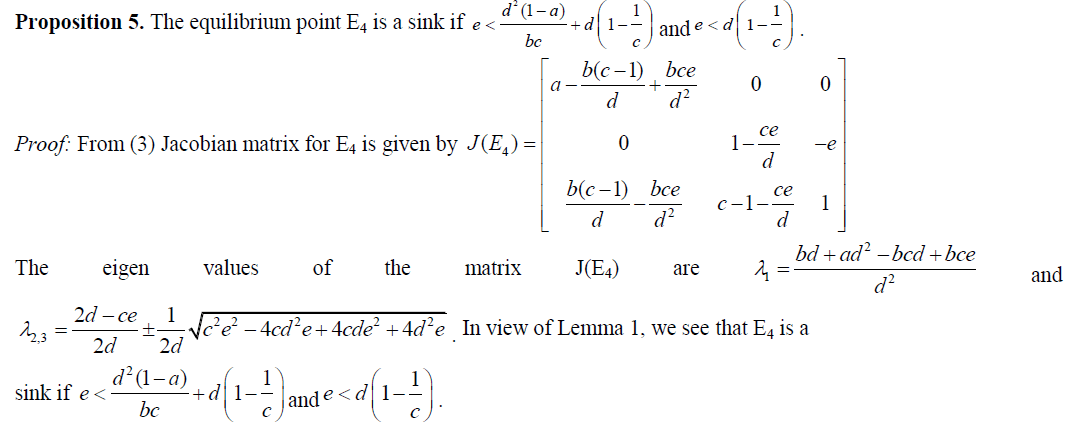
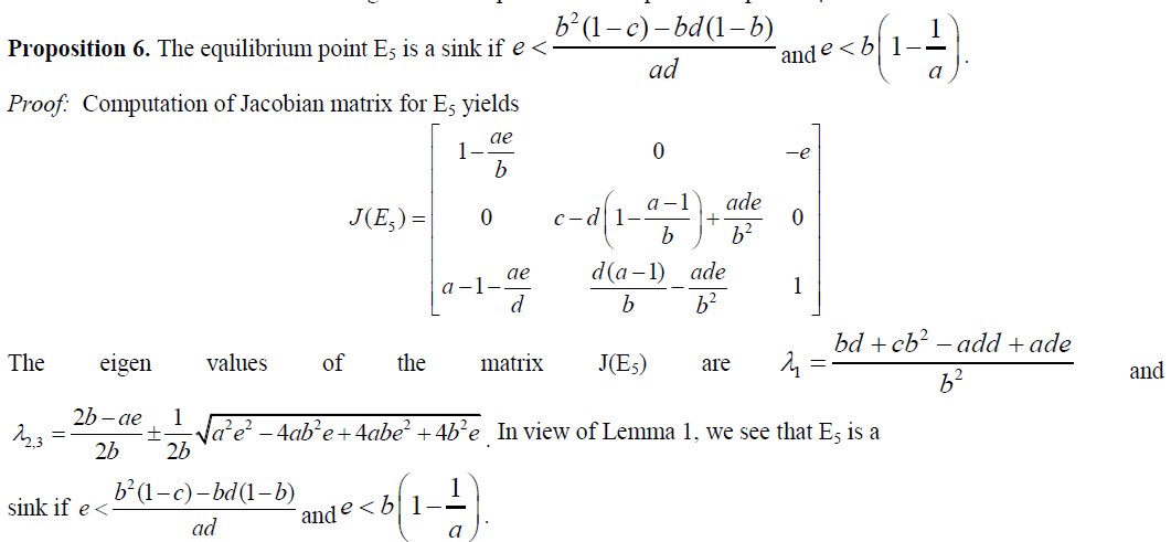
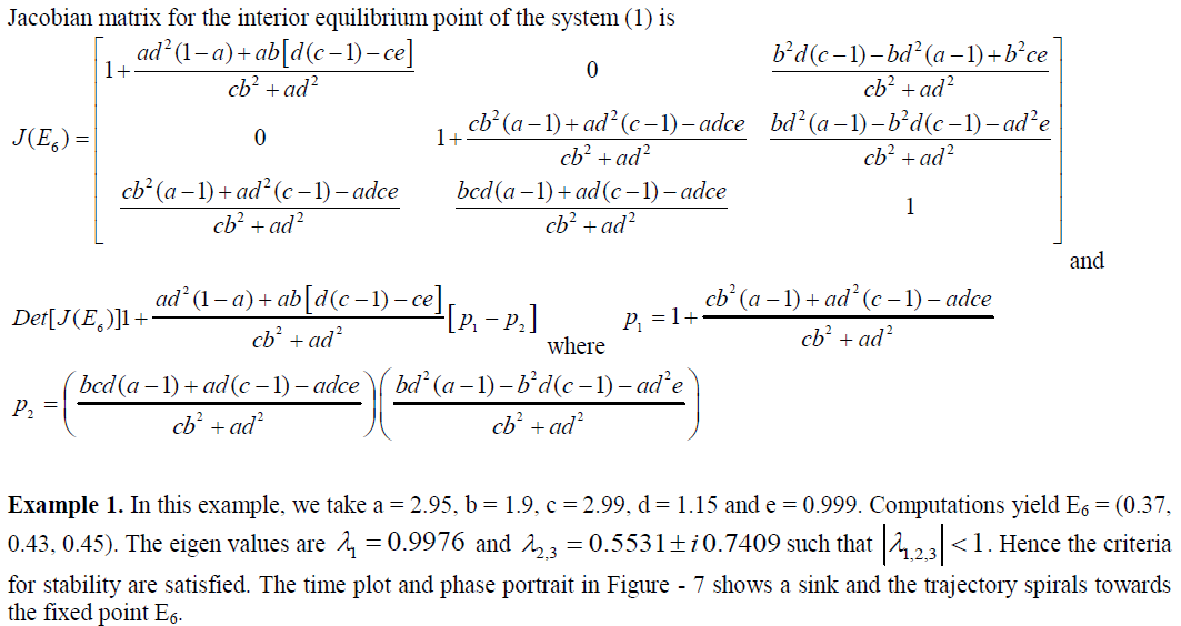
In this section, we provide numerical examples and simulations which help us to analyse the stability properties of the system (1) by graphing time plots for x(n), y(n), z(n) and phase diagrams. We consider ranges of the parameters provided by the analysis presented in the following propositions. The examples explain the complex dynamics of the system. The local stability analysis of the model can be carried out by computing the Jacobian corresponding to each equilibrium point and finding eigen values from the Jacobian matrix. The Jacobian matrix J for the system (1) has the form

VI. BIFURCATION DIAGRAMS

Bifurcation diagrams provide information about abrupt changes in the dynamics, see Figure-8. The parametric values at which these changes occur are called bifurcation points. They provide information about the dependence of the dynamics on a certain parameter. If the qualitative change occurs in a neighbourhood of an equilibrium point or periodic solution, it is called a local bifurcation. Any other qualitative change that occurs is considered as a global bifurcation.

Example 3. The parameters are assigned the values b = 1.88, c = 2.99, d = 0.99, e = 0.999 and the bifurcation diagram is plotted for the growth parameter in the range 3.0001 – 4.5. Both prey and predator population exhibit chaos.

References

1. [1] Abd-Elalim A. Elsadany, H. A. EL-Metwally, E. M. Elabbasy, H. N. Agiza, Chaos and bifurcation of a nonlinear discrete prey-predator system, Computational Ecology and Software, 2012,2(3):169-180.
2. [2] CananCelik, OktayDuman, Allee effect in a discrete-time predator prey system, Chaos, Solitons and Fractals, 40, (2009), 1956-1962.
3. [3] Leah Edelstein-Keshet, Mathematical Models in Biology, SIAM, Random House, New York, 2005.
4. [4] Marius Danca, StelianaCodreanu and Botond Bako, Detailed Analysis of a Nonlinear Prey-predator Model, Journal of Biological Physics 23: 1120, 1997.
5. [5] J.D.Murray, Mathematical Biology I: An Introduction, 3-e, Springer International Edition, 2004.
6. [6] Saber Elaydi, An Introduction to Difference Equations, Third Edition, Springer International Edition, First Indian Reprint, 2008.
7. [7] Temple H. Fay, Johanna C. Greeff, Lion, wildebeest and zebra: A predator–prey model, ecological modelling, 196(2006)237–244.
8. [8] M.ReniSagaya Raj, A.George Maria Selvam, R.Janagaraj, Dynamical Behaviour of Discrete Prey-Predator system with Scavenger, International Journal of Emerging Research in Management & Technology ISSN: 2278-9359 (Volume-2, Issue-11), November 2013, pp: 27 - 33.
9. [9] Robert M.May, Biological Populations with Non overlapping Generations: Stable Points, Stable Cycles and Chaos, Science, New Series, Vol.186, No.4164 (Nov. 15, 1974), 645 - 647.