A Hybrid Deep Learning Model for Space Radiation Dose Rate Prediction

Abstract

The prediction of space radiation dose rates holds significant importance for space science research. In this paper, a hybrid neural network-based approach for forecasting space radiation dose rates is proposed, utilizing a dataset of 4,174,202 in orbit measurements collected over a 12-month period from satellites. During data pre-processing, a first derivative wavelet transform is applied to retain trend information and perform noise reduction. In model design, the FDW-LSTM model is introduced, combining the First Derivative Wavelet (FDW) transform with Long Short-Term Memory (LSTM) networks. Experimental results demonstrate a coefficient of determination (R²) of 0.97 between the predicted values and actual measurements for the FDW-LSTM model. Compared to the Mean Absolute Deviation (MAD), 3-Sigma Rule (3σ), and Quartile methods, the FDW-LSTM model yields an average increase of 0.2 in R². Additionally, compared to the predictions of the GRU and RNN neural networks, the FDW-LSTM model achieves an improvement of 0.12 and 0.54 in R², respectively.

Keywords

Dose rate prediction; Network; Long Short-Term Memory (LSTM); Wavelet transform

Introduction

The space radiation environment significantly impacts satellite operations. Satellites in orbit are exposed to various forms of radiation such as protons, electrons and heavy ions, leading to single particle effects that can seriously affect their reliability. Dose rate, as a critical component of space radiation, holds undeniable importance. Accurate assessment of dose rates is crucial for a multitude of space science studies, ranging from investigating the impact of radiation on organisms to exploring space weather phenomena, all of which heavily rely on dose rate [1-7].

However, merely understanding the variations in the radiation environment falls short; accurate prediction is equally crucial. Precisely forecasting the changes in dose rate provides valuable data reference for satellite operational forecasting and space weather research. With the continuous advancement of the field of machine learning, many studies are applying deep learning to time series prediction, among which neural networks have exhibited strong performance in space radiation prediction. Given the data characteristics of radiation dose rates, methods such as Convolutional Neural Networks (CNN) and ARMA Neural Networks, which possess unique advantages in addressing time series problems, have also been employed for space radiation prediction, significantly enhancing predictive accuracy. Specifically, Long Short-Term Memory Networks (LSTM) have shown superior predictive performance in time series forecasting due to their distinctive forget gate mechanism [8-23]. Meysam et al. proposed a hybrid machine learning algorithm, WLSTM, for daily solar radiation prediction, considering relative humidity, potential evapotranspiration, temperature, precipitation, and temperature. The model was trained with five different input combinations, and the results indicated that the WLSTM model significantly improved predictive accuracy, with the worst R₂ value reaching 0.88 and the best R² achieving 0.966 [24]. Sahar et al. combined Support Vector Machine (SVM), Gene Expression Programming (GEP), Long Short-Term Memory Networks (LSTM), and wavelet transform for predicting solar radiation across five datasets [25]. The outcomes demonstrated that the results obtained using the LSTM model had lower dispersion and outperformed other models in terms of RMSE, SI, and MAE evaluation metrics. WEI, Lihang, et al. employed Long Short-Term Memory Networks (LSTM) to develop a model for predicting daily >2 MeV electron integral flux in the geostationary orbit [26]. Their model utilized geomagnetic and solar wind parameters as well as the past five days' values of >1 MeV electron integral flux itself as inputs. Experimental results indicated a significant improvement in predictive efficiency compared to some earlier models, with predictive efficiencies of 0.833, 0.896 and 0.911 for the years 2008, 2009 and 2010 respectively.

Overall, in the context of space radiation environment, particularly the prediction of space radiation dose rates, although machine learning methods offer a promising avenue, they also encounter a series of challenges. Firstly, the complexity of the data increases the difficulty of the prediction task. Secondly, the presence of various noise sources may interfere with predictive models, affecting the accuracy of predictions. Most importantly, the accuracy of the prediction model remains a critical challenge [27-31].

Due to the large volume of satellite measurement data, the space environment of on-orbit satellites is complex and dynamic. Additionally, factors such as detector technology and raw data unpacking techniques contribute to various forms of noise in the measured data. Therefore, employing suitable data preprocessing techniques to handle the measured data is crucial in obtaining data that is conducive to subsequent neural network learning [32].

Traditional data preprocessing methods, such as the Median Absolute Deviation (MAD) and the 3σ (standard deviation) method, incur high time costs and exhibit poor performance when applied to this type of data. Moreover, they may lead to the loss of the original data's trend. Consequently, there is a need for more effective time-series-based data preprocessing methods [33-37].

In recent years, wavelet decomposition, aimed at improving prediction accuracy, has garnered attention. Wavelet Transform (WT), a signal processing algorithm, is capable of beneficially decomposing observed time-series data in terms of both time and frequency. Wavelet analysis extracts information at different resolution levels from raw data, thereby enhancing the predictive performance of neural networks [38-42].

For instance, Sharifi et al. utilized Continuous Wavelet Transform (CWT) and Multi-Layer Perceptron Neural Network (MLPNN) to predict Solar Radiation (SR), resulting in favorable predictive performance [43]. The CWT-MLPNN combination displayed an improved correlation coefficient R₂ value from 0.86 to 0.89 for one-day-ahead prediction. Similarly, Singla et al. and associates proposed a model combining Full Wavelet Packet Decomposition (FWPD) with Bidirectional Long Short-Term Memory (BILSTM) [44]. This fusion raised the R₂ value for SR prediction from 0.918 to 0.999.

In summary, to further enhance the prediction accuracy of space radiation dose rates, this paper proposes a model that combines First Derivative Wavelet (FDW) and Long Short-Term Memory (LSTM), referred to as FDW-LSTM. The main contributions of this paper are as follows: (1) Introducing a data preprocessing method (First Derivative Wavelet Transform) to capture the trend of measured data, applying wavelet transform for noise reduction, and extracting valuable information. (2) Utilizing the LSTM neural network for predicting space radiation dose rates. (3) Through experimental comparisons, validating the accuracy of the proposed FDW-LSTM model, which outperforms traditional neural network models in predicting space radiation dose rates.

Materials and Methods

Data preparation

The in-orbit satellite dose rate data in this paper is provided by Shanghai Sast Space Technology Co. Ltd. The satellite number used in this paper is 52085, with orbital elements as follows: Semi-major axis of 7395 km, eccentricity of 0.01, inclination angle of 63.398, perigee argument of 41.145, right ascension of ascending node of 132.892, and mean anomaly of 319.739. The orbital period is 105.47 minutes. The satellite employs Si detectors with an equivalent shielding thickness of 1 mm Al. The dose rate data used in this study is selected from the satellite's measurements taken from April 2022 to March 2023.

In Table 1, the data is categorized into 26 operating cases. For each case, the provided information includes the time range, space weather event type and occurrence time.

Table 1. Detailed information of operating cases.

Table 2. Evaluation criteria after different wavelet basis processing.

Data pre processing

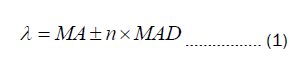
Currently, commonly used data processing methods include the Median Absolute Deviation (MAD) method, the 3σ (three times standard deviation) method, and the quartile method. MAD method, a frequently employed technique for outlier detection in recent years, exhibits characteristics of insensitivity to both sample size and outliers. The primary steps involved in this approach are as follows: Firstly, calculate the median MA of variable A; Secondly, subtract the median MA from variable A to obtain variable B and take the absolute value of variable B, yielding variable C; Thirdly, determine the median MC of variable C; Fourthly, transform MC into MAD, MAD=1.4862 × MC; Sixthly, compute the threshold λ , where values exceeding λ are considered outliers to be removed, according to the formula provided below, (where n represents a multiplier, chosen based on practical considerations):

The 3σ calculates the standard deviation and establishes a valid value range based on a certain probability. This method is applicable to data that follows a normal distribution and assumes a large dataset. According to this method, data falling within the range of (μ-3σ, μ+3σ) are considered normal values (where μ represents the mean and σ denotes the standard deviation), while data outside this range are identified as outliers and should be eliminated.

The quartile method entails the computation of three data points to partition a dataset into four equal segments. The precise steps for calculation are as follows: Firstly, determine the first quartile point Q₁ and the third quartile point Q3. Subsequently, calculate the Inter Quartile Range (IQR), which is defined as the difference between Q₃ and Q1, I_QR =Q₃- Q₁. Finally, data falling within the range of (Q₁-3I_QR, Q3+3I_QR) are regarded as normal values, whereas data points lying outside this range are identified as outliers and thus should be eliminated.

The aforementioned data processing methods involve removing data points based on predefined thresholds. While these methods can eliminate some outliers, these data points often hold significance in dose rate prediction. Removing such data points can disrupt the inherent trend of the original data, hindering subsequent neural networks from learning the complete time series pattern.

In the realm of time series analysis, the discovery of wavelet transform has introduced a novel technical approach for analyzing noise phenomena. Wavelets, being finite-length orthogonal bases, offer a means to represent time series in the domain of time scales at varying resolutions. This makes them particularly well-suited for decomposing non-stationary time series data.

In Figure 1, we employ the first derivative wavelet transform, a method capable of addressing the over-elimination issue during data preprocessing while preserving the original data's fluctuation trend. The process of the first derivative wavelet transform involves calculating the trend component of the data using the moving average method, decomposing the data through wavelet transform with appropriate wavelet bases and decomposition levels. This ultimately yields processed, reliable and accurate time series data.

Figure 1: Data preprocessing process (the first derivative wavelet transform).

We start by employing the moving average method to calculate the data's trend component, denoted as Tt. The moving average method is a commonly used smoothing technique that involves computing the mean of the data within a sliding window to reduce noise and retain trend information. By calculating the trend component, we can better capture the overall data trend, perform preliminary noise reduction, and minimize interference in subsequent analysis and modeling. The formula for the moving average method is as follows:

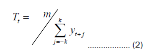
Where y_t represents the time series data, and m=2k+1, implying that the trend at time t is obtained by calculating the average of y_t over the preceding and succeeding k cycles. This approach is referred to as "m-MA," specifically "m-order moving average." In the case of achieving an even-order moving average, we perform two consecutive oddorder moving averages to accomplish this.

Next, we process the data using wavelet transform. To determine the threshold, we employ the technique of wavelet transform with the minimax threshold method. This approach relies on the distribution characteristics of wavelet coefficients and involves comparing the amplitude of wavelet coefficients to the threshold to identify anomalies. It is a straightforward and effective signal processing method, capable of efficiently removing noise while retaining crucial information. The threshold λ is calculated using the following empirical formula:

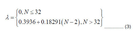
Where N represents the length of the input sequence.

Proposed neural network

Recurrent Neural Network (RNN) is a fundamental type of multi-layered feedback neural network that exhibits strong processing capabilities for sequential data. RNN can be represented by the following computational formula:

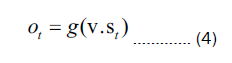
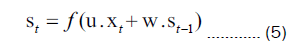
In Equation (4) and (5), the variable V signifies the weight parameters that connect the hidden layer to the output layer. The variable St represents the hidden layer values, which are determined by applying an activation function g to the weighted sum of the inputs. The output layer values Ot are obtained from the hidden layer values. The variable U represents the weight parameters connecting the input layer to the hidden layer. The variable X_t denotes the current input values, while S_t-1 represents the values of the previous hidden layer.

It is evident from the equation that the hidden layer values S_t not only depend on the current input values X_t but also take into account the influence of the previous hidden layer values S_t-1 weighted by W in the current input. This weighted contribution allows for the consideration of the previous hidden layer's impact on the current hidden layer values.

The Gated Recurrent Unit (GRU) introduces the concepts of an update gate and a reset gate in order to better retain historical information. The computation formula for GRU is as follows:

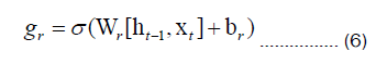
In Eq. (6), gr corresponds to the gate control vector of the reset gate, which is determined based on the current input x_t and the state vector from the previous time step h_t-1. The sigmoid activation function σ is applied, and W_r and b_r represent the weights and biases associated with the reset gate.

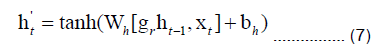
In Equation. (7), the variable h'_t represents the candidate state at time step t. It is computed by activating the reset gate gr and the state vector from the previous time step h_t-1 using the tangent (tanh) function. The weights and biases related to the candidate state are denoted as W_h and b_h.

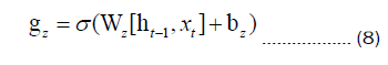
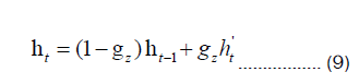
Equations 8 and 9 introduce the use of gz to control the signal of the new input state vector h'_t .On the other hand, 1-gz is utilized to regulate the influence of the previous time step's state vector h_t-1 on the new input state vector h'_t . These gating mechanisms serve to control the impact of the previous time step's state vector on the computation of the new input state vector.

LSTM represents a refined version of traditional RNN. While conventional RNN process input and output sequences independently, they encounter challenges in capturing intricate relationships within long sequences, where the interdependencies between earlier and later segments are crucial. Consequently, LSTM was introduced as a solution to address the issue of long-term dependencies within time series data. By virtue of its advanced memory capabilities, LSTM excels in acquiring and retaining long-term dependencies, thus facilitating the seamless propagation of information across multiple time steps in a time series. Notably, LSTM surpasses RNN in terms of performance when confronted with extensive sequences.

Figure 2 depicts the structure of the LSTM model, comprising three LSTM layers labeled as A. Each LSTM layer incorporates distinct neuron inputs, namely the current input Xt, the output of the preceding LSTM unit h_t-1, and the cell state vector of the preceding LSTM unit C_t-1. The neuron outputs of each LSTM layer encompass the output of the current LSTM unit Ht and the cell state vector of the current LSTM unit at time step t, represented as C_t.

Figure 2: Structure of LSTM model.

The internal neural architecture of LSTM, consists of memory cells within each layer. These memory cells incorporate essential components such as the forget gate f_t, input gate i_t, and output gate O_t. The forget gate plays a crucial role in deciding the information to be discarded or preserved. By subjecting the current input X_t and the output of the previous LSTM unit h_t-1 to a sigmoid activation function, a range of values between 0 and 1 is obtained. Values close to 1 signify the information to be retained, while values close to 0 indicate the information to be forgotten. The expression for the forget gate can be expressed as:

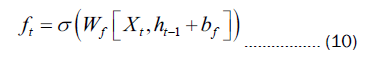
In Equation 10, W_frepresents the weights of the forget gate, and b_f represents the bias of the forget gate. The input gate serves to update the cell state within the LSTM network. Initially, the current input Xt and the output of the previous LSTM unit h_t-1 undergo a sigmoid activation function, resulting in a control value it ranging between 0 and 1.A value close to 0 signifies insignificance, whereas a value close to 1 denotes significance. Subsequently, the combination of the current input it and the output of the preceding LSTM unit h_t-1is fed into a tangent (tanh) function, producing a new state information that spans the range of 0 to 1. Essentially, encapsulates the pertinent information for the current LSTM unit, with it regulating the extent to which information from is assimilated into the cell state. Consequently, the previous cell state

C_t-1 Updated to the new cell state C_t by multiplying it with the forget gate f_t , which discards irrelevant information, and subsequently multiplying it with the input gate i_t and to yield the updated cell state vector:

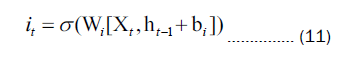
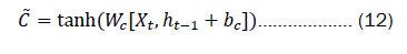
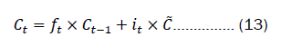
In Equation 11 and 12, Wi and bi represent the weights and biases of the input gate, while Wc and bc represent the weights and biases of the control unit. The output gate serves the purpose of determining the value of the next hidden state. Initially, the sigmoid activation function is employed to ascertain the components of the cell state that should contribute to the output. Subsequently, the newly acquired cell state Ct from the input gate is subjected to the tangent (tanh) function. Ultimately, the output of the tanh function is multiplied by the output of the sigmoid activation function, yielding the ultimate output value Ct. The expression for this is as follows:

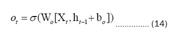
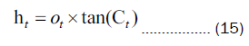
In Equation 14, Wo and bo represent the weights and biases of the output gate, respectively.

Evaluation criteria

Fifteen sets of data were randomly selected from the 26 different operating cases for training the data-driven model, while the remaining eleven sets were reserved for validation in each prediction. In order to mitigate the impact of randomness in training and testing set selection, as well as the variability introduced by parameter determination in modeling approaches, each method was run a minimum of 50 times to capture its predictive accuracy. The evaluation metrics were calculated using predicted data from the validation set and actual data.

To evaluate the predictive performance of the proposed model, three evaluation metrics are employed: The coefficient of determination (R²), Mean Squared Error (MSE), and Mean Absolute Error (MAE). The specific formulas for these metrics are as follows:

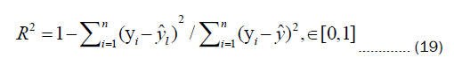
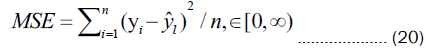
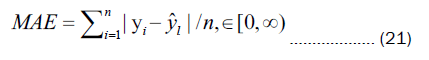
Where y_i represents the real value represents the predicted value represents the mean value of the real values, and n denotes the number of samples.

Results and Discussion

First Derivative Wavelet (FDW) method

To begin, the moving average method is employed to extract the trend component from the original dose rate data. In order to determine the appropriate order (m) for the moving average, this study examines orders of 2, 5, 7, and 9. The trend component curves obtained through the moving average method capture the primary direction of the time series. Furthermore, with increasing m, the moving average curve tends to become smoother. Since the moving average method provides an initial estimation of the trend component from the raw data and aims to retain the underlying fluctuation pattern, in this paper, we take m=2 (Figure 3).

Figure 3: Processing results of moving average method (m=2,5,7,9).

The second step involves denoising the trend component. We attempted denoising using five different wavelet bases: Haar, db2, db3, db4 and db5. Since excessively high decomposition levels can lead to the loss of some original signal information, all five wavelet bases were applied with a decomposition level of 1.

Table 2 presents the R₂ and MSE values after applying different wavelet bases for wavelet transformation. Upon comparison, it is evident that there is minimal variation in R₂ and only slight differences in MSE across these wavelet bases. This suggests that these wavelet bases possess similar capabilities in capturing data trends. Notably, the R₂ values for each wavelet base remain above 0.99, indicating the effectiveness of wavelet processing in preserving valuable information from the original data and retaining high-quality data points.

By comparing the effects of different wavelet bases, we obtained the results of the wavelet transformation. Among these wavelet bases, we observed that high decomposition levels lead to information loss. For our dataset, utilizing the db3 wavelet base is sufficient to achieve the desired outcome while retaining the essential fluctuation trends of the parent time series (Figure 4).

Figure 4: The results of different wavelet basis processing at different dose rate with respective time.

LSTM model structure and parameters

The structure and hyperparameters of the neural network model have a significant impact on its predictive performance. The structure involves factors such as the number of hidden layers and neurons per layer, while hyperparameters include batch size and number of iterations. In this study, a two-layer LSTM model was employed, with each layer containing 30 neurons. The batch size was set at 50, and the model was trained for 30 epochs. The model architecture is illustrated. The input data for the LSTM model consisted of preprocessed data, with the input factor being the univariate dose rate time series. The time step was set to 3. The Adam optimizer was used for optimization, and the training-to-testing dataset ratio was 0.5. To mitigate overfitting, a dropout layer with a dropout rate of 0.6 was introduced between the two LSTM layers. Finally, the predicted dose rate results were output through a fully connected layer (Figure 5).

Figure 5: Structure and hyperparameters of the neural network model of the LSTM.

To facilitate comparative analysis of the proposed model's predictive performance in subsequent experiments, this study conducts a comparison between the predictions of the LSTM model and those of the RNN and GRU models. The neural network architectures of the RNN and GRU models closely resemble that of the LSTM model, and the training and testing dataset divisions are consistent across all three models.

Experiments and analysis

Firstly, the initial set of experiments is conducted to analyze the impact of different data processing methods on predictive performance. The experimental results, revealing that the data processed using the FDW method demonstrates improved predictive performance in terms of MSE and MAE compared to the other three methods. Furthermore, the LSTM model based on the first derivative wavelet denoising method achieves a correlation coefficient of 0.94 between predicted and actual values, surpassing the performance of the LSTM model using other data processing techniques by enhancements of 0.15, 0.25 and 0.05, respectively. The primary reason for these differences lies in the FDW method's ability to retain high-quality data points from the original dataset while capturing the fluctuation trends through trend term estimation, resulting in a more accurate alignment of predictive outcomes with actual values (Table 3).

Table 3. Evaluation metrics for dose rate prediction of the LSTM model based on the FDW method, MAD method, 3σ method, and Quartile method.

Figure 6 illustrates the predictive results based on the FDW method, MAD method, 3σ method, and Quartile method using the LSTM model for operating condition #7. In the figure, the black line represents the actual dose rate values, while the red line represents the predicted values. From Figure 8, it can be observed that the MAD method exhibits the poorest predictive performance. This is attributed to the insensitivity of the MAD method to peak values in the data, rendering it unsuitable for handling the dose rate data in this study. The Quartile method displays a delayed response in its predicted values, coupled with suboptimal predictive performance.

Figure 6: Comparison of dose rate prediction using LSTM models with (a) FDW, (b) MAD, (c) 3σ, and (d) Quartile methods (case #7).

The 3σ method shows good numerical predictions, yet instances of predicted values exceeding actual values are evident, which is a recurring pattern in predictions across various conditions. The continuous occurrence of predicted values exceeding the actual values suggests that the model may have over fit the noise present in the training data and failed to accurately capture the true underlying relationship. Additionally, the 3σ method also demonstrates prediction delays. The subpar predictive accuracy of these methods arises due to their inability to eliminate a significant portion of noise, resulting in the neural network learning from noise during training and thus yielding inaccurate predictions. Moreover, both the MAD method and the 3σ method exhibit lagged predictions, stemming from the neural network's inability to effectively capture data trends.

In contrast, the FDW-LSTM model outperforms the other three models in numerical prediction and data fluctuation forecasting. This is attributed to the FDW method's initial trend term estimation during data processing, which maximally preserves data fluctuation trends. This enables the LSTM model to accurately capture data trends during subsequent learning, preventing misalignment between predicted and actual values. The FDW method's use of wavelet transformation aids in noise reduction and decomposition of the original time-series signal into sub-signals of different frequency components, facilitating the extraction of local features and trend information. This empowers the subsequent neural network model to learn from a cleaner time-series, focusing more effectively on useful information for prediction.

The final outcome underscores the FDW-LSTM model's capability to forecast dose rate data trends, with a correlation coefficient of 0.94 between predicted and actual values. This heightened accuracy results in improved predictive performance, achieving a more robust prediction outcome.

Moving on to the second set of experiments, we contrasted the predictive performance of different neural network models on dose rates. Both LSTM and GRU models utilized the FDW method for data pre-processing, as did the RNN model. The experimental results are presented. Analysis revealed that the LSTM model exhibited the lowest MSE, while both the LSTM and GRU models displayed similar MAE values, both of which were superior to the RNN model. The correlation coefficient R₂ between predicted and actual values was highest for the LSTM model, reaching 0.96. This is an improvement of 0.12 and 0.54 compared to the other two models, indicating that the LSTM model holds a advantage over the other neural network models in predicting dose rates within the space radiation environment (Table 4).

Table 4. Evaluation metrics for dose rate prediction of LSTM, GRU, and RNN models.

Figure 7 illustrates the best and worst predictive accuracy cases within the validation set. In the most favorable case (case ^#13), the FDW-LSTM model achieves an R² of 0.98, while in the least favorable case (case ^#16), the determination coefficient between FDW-LSTM model predictions and simulated data stands at 0.91. The black line represents satellite-measured dose rate data, the red line depicts FDW-LSTM model predictions, the green line signifies RNN model predictions, and the blue line indicates GRU model predictions.

Figure 7: Comparison diagram of dose rate prediction of LSTM, GRU and RNN models (The prediction of case #13 is the best (a), and the prediction of case #16 is the worst (b))

Overall, the FDW-LSTM model outperforms the other two models in both numerical prediction and capturing fluctuation trends. Particularly, in instances where the measured data values are on the higher side, FDW-LSTM demonstrates superior predictive performance compared to the other two models. However, there is room for improvement in accurately predicting peak values, which constitutes our next area of focus.

In Figure 7b the FDW-LSTM model avoids the misalignment of predicted and actual values. This is attributed to the FDW-LSTM model retaining the trend components of measured data during data preprocessing, allowing the trend of predicted values to closely match that of actual measurements.

Figure 8 showcases several scenarios from the validation set that encompass space weather events (case^#6, case^#10, case^#11, case^#21), including solar proton events and Relativistic Electron Enhancement. During occurrences of space weather phenomena, the model exhibits favorable predictive performance, thereby affirming its accuracy during space weather periods. Even amidst intense variations in the space environment, the FDW- LSTM model maintains a reasonable level of prediction accuracy. This capability offers a certain degree of predictive support for further space weather forecasting, particularly during periods of heightened space environmental activity.

Figure 8: The prediction performance of FDW-LSTM model during space weather.

Figure 9a displays the scatter plot of predicted values versus actual values obtained from the FDW-LSTM model for all scenarios, with the red lines representing an 8% error range. Observing the high-density points within the two red line regions demonstrates that the predictive errors of the FDW-LSTM model are well-contained within a reasonable range. However, a few data points still exhibit larger errors, necessitating further investigation to enhance the model's predictive accuracy. Moving, a numerical assessment of the FDW-LSTM model's predictive accuracy is presented. Figure 9b showcases the coefficient of determination (R²) between the predicted and actual values after predicting for all 26 scenarios. For the best-case scenario, the R² value between predicted and actual values reaches 98%. Conversely, for less favorable scenarios, the R² value between predicted and actual values is 91%. The average R² value across all 26 scenarios is 0.975, indicating a certain level of reliability in the predictive results. This further underscores the feasibility of the FDW-LSTM model proposed in this paper for predicting space radiation dose rates.

Figure 9: The two-dimensional scatter plot (a) of the predicted values and the measured values of the FDW-LSTM model for all cases and the correlation (b) between the predicted values and the measured values.

Conclusion

This paper proposes a model that combines the First Derivative Wavelet denoising (FDW) method with the Long Short-Term Memory (LSTM) neural network, referred to as the FDW-LSTM model. The innovation of this study lies in its exploration of a deep learning-based predictive model for space radiation dose rates. Furthermore, another novel aspect is the application of the FDW method in data pre-processing, which preserves the fluctuation of the original data while enhancing the dataset's suitability for neural network learning. The experimental findings lead to the following conclusions:

(1) The FDW method effectively denoises the original data and preserves the inherent fluctuation trend, as evidenced by an R₂ value of 0.98 between the FDW-processed data and the original data.

(2) The data processed with the FDW method yields improved predictive performance in the LSTM model, with an R² value of 0.96 between predicted and actual values. This represents a 20% average enhancement in R² value compared to the MAD method, quartile method, and 3σ method

(3) The FDW-LSTM model outperforms the GRU and RNN neural network models in predicting radiation dose rates, achieving an average R² value of 0.97. This marks a respective increase of 0.12 and 0.54 compared to the other two neural network models.

(4) The FDW-LSTM model attains an R² value of 0.91 even under the worst-case scenario, with an average accuracy of 0.97, demonstrating better predictive performance.

Therefore, the FDW-LSTM model holds a distinct advantage in predicting space radiation dose rates. The predictive data provided by this approach can offer support in space science research, such as space weather forecasting. While the neural network-based approach proves advantageous in adapting to data and uncovering underlying temporal features, addressing extreme cases (such as sudden magnitude shifts in dose rates) remains a challenging task, despite its ability to predict data fluctuation trends.

In conclusion, the FDW-LSTM model presents a viable solution for space radiation dose rate prediction, with the potential to support various applications in space science research, particularly in the realm of space weather prediction. Nonetheless, addressing exceptional circumstances that deviate significantly from the norm, while predicting fluctuation trends, remains a challenging aspect of this neural network-based method.

Credit Authorship Contribution Statement

Zhiqian Zhang: Calculations and writing. Yuxiong Xue: conceptualization and methodology. Xianghua Zeng: conceptualization, methodology, writing – review & editing, and supervision.

All authors read and approved the final manuscript.

Acknowledgement

This work was supported by the National Natural Science Foundation of China (61474096), the Yangzhou Science and Technology Bureau (YZ2020263), Open Project of State Key Laboratory of Intense Pulsed Radiation Simulation and Effect (SKLIPR2115) and Foundation of National Key Laboratory of Materials Behavior and Evaluation Technology in Space Environment (WDZC-HGD-2022-11).

Data Availability

The datasets used and analysed during the current study are available from the corresponding author on reasonable request.

Decalaration of Competing Interest

The authors declare that they have no known competing financial interests or personal relationships that could have appeared to influence the work reported in this paper.

References

1. Baker DN, et al. Relativistic electron acceleration and decay time scales in the inner and outer radiation belts: SAMPEX. Geophys Res Lett. 1994;21.6:409-412.

   [Crossref] [Google Scholar]

2. Pilipenko V, et al. Statistical relationships between satellite anomalies at geostationary orbit and high-energy particles. ASR. 2006;6:1192-1205.
3. Tabocchini MA. A forty-year journey from “classical” biophysics and radiobiology to hadrontherapy, space radiation and low dose rate underground radiobiology. Int J Radiat Biol. 2022;3:383-394.

   [Crossref] [Google Scholar]

4. Acharya MM, et al. Erratum: Acharya et al., new concerns for neurocognitive function during deep space exposures to chronic, low dose-rate, neutron radiation. eNeuro. 2019;5:ENEURO.0367-ENEU19.2019.

   [Crossref] [Google Scholar]

5. Pei W, et al. Current status of space radiobiological studies in China. Life Sci Space Res. 2019;22:1-7.

   [Crossref] [Google Scholar]

6. Kauristie K, et al. Space weather services for civil aviation—Challenges and solutions. Remote Sensing. 2021;18:3685.

   [Crossref] [Google Scholar]

7. Bain HM, et al. Improved space weather observations and modeling for aviation radiation. Front Astron Space Sci. 2023;10:54.

   [Crossref] [Google Scholar]

8. Fabian X, et al. Artificial neural networks for neutron/γ discrimination in the neutron detectors of NEDA. Nucl Instrum Methods Phys Res A: Accel Spectrom Detect Assoc Equip. 2021;986:164750.

   [Crossref] [Google Scholar]

9. Bae JW, et al. Reconstruction of fast neutron direction in segmented organic detectors using deep learning. Nucl Instrum Methods Phys Res A: Accel Spectrom Detect Assoc Equip. 2023; 1049:168024.

   [Crossref] [Google Scholar]

10. Wang H, et al. Detecting ship targets in spaceborne infrared image based on modeling radiation anomalies. Infrared Phys Technol. 2017;85:141-146.

    [Crossref] [Google Scholar]

11. Dadu KS, et al. Multistep lead time forecasting of hydrologic time series using daubechies wavelet-neural network hybrid model. Int j sci eng res. 2013;10:115-124. 

    [Google Scholar]

12. Qin M, et al. Red tide time series forecasting by combining ARIMA and deep belief network. KBS. 2017;125:39-52. [Crossref]

    [Google Scholar]

13. Sun H, et al. Empirical investigation on modeling solar radiation series with ARMA–GARCH models. Energy Convers Manag. 2015;92:385-395.

    [Crossref] [Google Scholar]

14. Miow XC, et al. Demand response for frequency regulation with neural network load controller under high intermittency photovoltaic systems[J]. Energy Rep. 2023;9:2869-2880.

    [Crossref] [Google Scholar]

15. Antoni R, et al. Prediction of fast neutron spectra with a spherical TEPC using a machine-learning algorithm. Nucl Instrum Methods Phys Res A: Accel Spectrom Detect Assoc Equip. 2023;1050:168139.

    [Crossref] [Google Scholar]

16. Ma Y, et al. Recurrent neural networks for discrimination of exo-atmospheric targets based on infrared radiation signature. Infrared Phys Technol. 2019;96:123-132.

    [Crossref] [Google Scholar]

17. Bamisile O, et al. Comparison of machine learning and deep learning algorithms for hourly global/diffuse solar radiation predictions. Int J Energy Res. 2022;8:10052-10073.

    [Crossref] [Google Scholar]

18. Fortino GF, et al. Digital signal analysis based on convolutional neural networks for active target time projection chambers. Nucl Instrum Methods Phys Res A: Accel Spectrom Detect Assoc Equip. 2022;1031:166497. [Crossref]

    [Google Scholar]

19. Zhang S, et al. Spatial infrared objects discrimination based on multi-channel CNN with attention mechanism. Infrared Phys Technol. 2023;132:104670.

    [Crossref] [Google Scholar]

20. David M, et al. Probabilistic forecasting of the solar irradiance with recursive ARMA and GARCH models. Solar Energy. 2016;133:55-72.

    [Crossref] [Google Scholar]

21. Mirzaei M, et al. A novel stacked long short-term memory approach of deep learning for streamflow simulation. Sustainability. 2021;23:13384.

    [Google Scholar]

22. Wielgosz M, et al. Using LSTM recurrent neural networks for monitoring the LHC superconducting magnets. Nucl Instrum Methods Phys Res. 2017;867:40-50.

    [Crossref] [Google Scholar]

23. Zhao F, et al. Exo-atmospheric infrared objects classification based on dual channel LSTM network. Infrared Phys Technol. 2020;111:103535.

    [Google Scholar]

24. Alizamir M, et al. Improving the accuracy of daily solar radiation prediction by climatic data using an efficient hybrid deep learning model: Long short-term memory (LSTM) network coupled with wavelet transform. Eng Appl Artif Intell. 2023;123:106199.

    [Crossref] [Google Scholar]

25. Mohsenzadeh S et al. Hybrids of machine learning techniques and wavelet regression for estimation of daily solar radiation. Stoch Environ Res Risk Assess. 2022;12:4255-4269.

    [Crossref]

26. Wei L, et al. Quantitative prediction of high‐energy electron integral flux at geostationary orbit based on deep learning. Space Weather. 2018;7:903-916.

    [Crossref] [Google Scholar]

27. Ginet GP, et al. Proton flux anisotropy in low earth orbit. IEEE Transactions on Nuclear Science. 2007;6:1975-1980.

    [Crossref] [Google Scholar]

28. Nagatsuma T, et al. Space environment data acquisition monitor onboard Himawari-8 for space environment monitoring on the Japanese meridian of geostationary orbit. Earth Planets Space. 2017.

    [Crossref] [Google Scholar]

29. Turhan B. On the dataset shift problem in software engineering prediction models. Empir Software Eng. 2012;17:62-74.

    [Crossref] [Google Scholar]

30. Sajid M, et al. Space radiation environment prediction for VLSI microelectronics devices onboard a LEO satellite using OMERE-TRAD software. ASR. 2015; 2:314-324. 

    [Google Scholar]

31. Lin ZW, et al. Comparisons of several transport models in their predictions in typical space radiation environments. ASR. 2012;4:797-806. [Crossref]

    [Google Scholar]

32. Sihver L, et al. Space radiation risk reduction through prediction, detection and protection. In: 2021 IEEE aerospace conference (50100). IEEE. 2021;p:1-10.

    [Crossref]

33. Tao Y, et al. Empirical wavelet transform method for GNSS coordinate series denoising. J geovis spat anal. 2021;5:1-7.

    [Crossref]

34. Jamei M, et al. Designing a decomposition-based multi-phase preprocessing strategy coupled with EDBi-LSTM deep learning approach for sediment load forecasting. Ecol Indic. 2023;153:110478.

    [Crossref] [Google Scholar]

35. Yitzhaki S, et al. The relationship between the absolute deviation from a quantile and Gini’s mean difference. METRON. 2013;71:97-104.

    [Crossref] [Google Scholar]

36. Majumder A, et al. Standard deviation method based pso: an instigated approach to optimize multi-objective manufacturing process parameters[J]. Int J Swarm Intell Res (IJSIR). 2016;7:15-35.

    [Crossref] [Google Scholar]

37. Leys C, et al. Detecting outliers: Do not use standard deviation around the mean, use absolute deviation around the median. J Exp Soc Psychol. 2013;4:764-766.

    [Crossref] [Google Scholar]

38. Belkadhi K, et al. Dose calculation using a numerical method based on Haar wavelets integration. Nucl Instrum Methods Phys Res A: Accel Spectrom Detect Assoc Equip. 2016;812:73-80.

    [Crossref] [Google Scholar]

39. Sullivan CJ, et al. Generation of customized wavelets for the analysis of γ-ray spectra. Nucl Instrum Methods Phys Res A: Accel Spectrom Detect Assoc Equip. 2007;1:275-278.

    [Crossref] [Google Scholar]

40. Ma X, et al. A TFA-CNN method for quantitative analysis in infrared spectroscopy. Infrared Phys Technol. 2022;126:104329.

    [Crossref]

41. Gu L, et al. Enhancement method of weak Lidar signal based on adaptive variational modal decomposition and wavelet threshold denoising. Infrared Phys Technol. 2022;120:103991.

    [Crossref] [Google Scholar]

42. Liu J, et al. Improvement of the fast simulation of gamma-gamma density well logging measurement. Appl Radiat Isot. 2021;167:109423.

    [Crossref] [Google Scholar]

43. Sharifi SS, et al. Multi-time-step ahead daily global solar radiation forecasting: performance evaluation of wavelet-based artificial neural network model. Meteorol Atmos Phys. 2022;3:50.

    [Crossref] [Google Scholar]

44. Singla P, et al. A hybrid solar irradiance forecasting using full wavelet packet decomposition and bi-directional long short-term memory (BiLSTM). Arab J Sci Eng. 2022;11:14185-14211.

    [Crossref] [Google Scholar]