Keywords
|
| Digital Image Processing, Mat lab. |
INTRODUCTION
|
| In image processing it is usually necessary to perform high degree of noise reduction in an image before performing higher-level processing steps, such as edge detection. The median filter is a non-linear digital filtering technique, often used to remove noise from images or other signals. The idea is to examine a sample of the input and decide if it is representative of the signal. This is performed using a window consisting of an odd number of samples. The values in the window are sorted into numerical order; the median value, the sample in the center of the window, is selected as the output. The oldest sample is discarded, a new sample acquired, and the calculation repeats. A new framework for removing impulse noise from images is presented in which the nature of the filtering operation is conditioned on a state variable defined as the output of a classifier that operates on the differences between the input pixel and the remaining rank-ordered pixels in a sliding window. As part of this framework, several algorithms are examined, each of which is applicable to fixed and random-valued impulse noise models. First, a simple two-state approach is described in which the algorithm switches between the outputs of mean filter. |
| This paper is an enhancement to our earlier research with grey-scale images. In this paper, we propose two new detection-estimation based image filtering algorithms that effectively remove corrupted pixels with impulsive noise in digital color images. The existing methods for enhancing corrupted color images typically possess inherent problems in computation time and smoothing out edges because all pixels are filtered. Our proposed algorithms first classify corrupted pixels in each channel or in each pixel. Because marginal or vector median filtering is only performed for the classified pixels, the process is computationally efficient, and edges are preserved well. In addition, because there is no appropriate criterion to evaluate the performance of impulsive noise detectors for color images, the objective comparison of noise detectors is difficult. Thus, we introduce a new efficiency factor for comparing the performance of noise detectors in digital color images. |
| Necessary and sufficient conditions for a signal to be invariant under a specific form of median filtering are derived. These conditions state that a signal must be locally monotone to pass through a median filter unchanged. It is proven that the form of successive median filtering of a signal (i.e., the filtered output is itself again filtered) eventually reduces the original signal to an invariant signal called a root signal. For a signal of length L samples, a maximum of i (L - 2) repeated filtering produces a root signal. |
Block Diagram
|
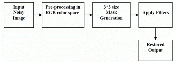 |
NOISE AND FILTERS
|
| Noise: In common use the word noise means unwanted sound or noise pollution. In electronics noise can refer to the electronic signal corresponding to acoustic noise (in an audio system) or the electronic signal corresponding to the (visual) noise commonly seen as 'snow' on a degraded television or video image. In signal processing or computing it can be considered data without meaning; that is, data that is not being used to transmit a signal, but is simply produced as an unwanted by-product of other activities. In Information Theory, however, noise is still considered to be information. In a broader sense, film grain or even advertisements in web pages can be considered noise. |
| Noise Generation: Noises are random background events which have to be dealt with in every system processing real signals. They are not part of the ideal signal and may be caused by a wide range of sources, e.g. variations in the detector sensitivity, environmental variations, the discrete nature of radiation, transmission or quantization errors, etc. It is also possible to treat irrelevant scene details as if they were image noise (e.g. surface reflectance textures). The characteristics of noise depend on their source, as does the operator which best reduces their effects. Many image processing packages contain operators to artificially add noise to an image. Deliberately corrupting an image with noise allows us to test the resistance of an image processing operator to noise and assess the performance of various noise filters. |
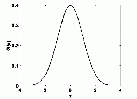
| Detector Noise: One kind of noise which occurs in all recorded images to a certain extent is detector noise. This kind of noise is due to the discrete nature of radiation, i.e. the fact that each imaging system is recording an image by counting photons. Allowing some assumptions (which are valid for many applications) this noise can be modeled with an independent, additive model - where the noise n (i, j) has a zero-mean Gaussian distribution described by its standard deviation (σ), or variance. (The 1-D Gaussian distribution has the form shown in Figure 1.) This means that each pixel in the noisy image is the sum of the true pixel value and a random, Gaussian distributed noise value. |
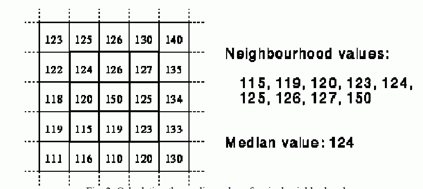
| Median Filter: The median filter is normally used to reduce noise in an image, somewhat like the mean filter. However, it often does a better job than the mean filter of preserving useful detail in the image. Like the mean filter, the median filter considers each pixel in the image in turn and looks at its nearby neighbours to decide whether or not it is representative of its surroundings. Instead of simply replacing the pixel value with the mean of neighboring pixel values, it replaces it with the median of those values. The median is calculated by first sorting all the pixel values from the surrounding neighbourhood into numerical order and then replacing the pixel being considered with the middle pixel value. (If the neighbourhood under consideration contains an even number of pixels, the average of the two middle pixel values is used.) Figure 1 illustrates an example calculation. |
| In the above Fig. 2 As can be seen the central pixel value of 150 is rather unrepresentative of the surrounding pixels and is replaced with the median value: 124. A 3×3 square neighborhood is used here --- larger neighborhoods will produce more severe smoothing. |
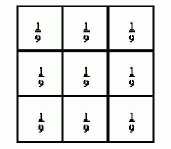
| Mean Filter: Mean filtering is a simple, intuitive and easy to implement method of smoothing images, i.e. reducing the amount of intensity variation between one pixel and the next. It is often used to reduce noise in images. The idea of mean filtering is simply to replace each pixel value in an image with the mean (`average') value of its neighbors, including itself. This has the effect of eliminating pixel values which are unrepresentative of their surroundings. Mean filtering is usually thought of as a convolution filter. Like other convolutions it is based around a kernel, which represents the shape and size of the neighborhood to be sampled when calculating the mean. Often a 3×3 square kernel is used, as shown in Figure 1, although larger kernels (e.g. 5×5 squares) can be used for more severe smoothing. (Note that a small kernel can be applied more than once in order to produce a similar - but not identical - effect as a single pass with a large kernel.) |
| Computing the straightforward convolution of an image with this kernel carries out the mean filtering process. |
METHODOLOGY FOR NOISE REMOVAL IN DIGITAL IMAGES
|
| In our project, two different image filtering algorithms are compared based on their ability to reconstruct noise affected Images. The purpose of these algorithms is to remove noise from a signal that might occur through the transmission of an image. |
Noise Generation:
|
| In testing, we consider sets of images containing various amounts of artificial noise. Impulse noise represents random spikes of energy that happen during the data transfer of an image. To generate noise, a percentage of the image is damaged by changing a randomly selected point channel to a random value from 0 to 255. The noise model, In, is given by |
 |
| where I is the original image, Ir, Ig, and Ib represent the original red, green, and blue component intensities of the original image, x,y= [0,1] are continuous uniform random numbers, z= [0,255] is a discrete uniform random number, and p = [0,1] is a parameter which represents the probability of noise in the image. |
Mean Filter Technique:
|
| The simplest of these algorithms is the Mean Filter. The Mean Filter is a linear filter which uses a mask over each pixel in the signal. Each of the components of the pixels which fall under the mask are averaged together to form a single pixel. This new pixel is then used to replace the pixel in the signal studied. The Mean Filter is poor at maintaining edges within the image. |
 |
Median Filter Technique:
|
| The use of the median in signal processing was first introduced by J. W. Tukey. The Median Filter is performed by taking the magnitude of all of the vectors within a mask and sorting the magnitudes. The pixel with the median magnitude is then used to replace the pixel studied. The Simple Median Filter has an advantage over the Mean filter in that it relies on median of the data instead of the mean. A single noisy pixel present in the image can significantly skew the mean of a set. The median of a set is more robust with respect to the presence of noise. |
 |
| When filtering using the Simple Median Filter, an original pixel and the resulting filtered pixel of the sample studied are sometimes the same pixel. A pixel that does not change due to filtering is known as the root of the mask. It can be shown that after sufficient iterations of median filtering every signal converges to a root signal. |
EXPERIMENTAL RESULTS COMPARISONS
|
| To test the accuracy of the Mean and Median Filters, we need three things: an uncorrupted image, the image with corruption applied by some means, and the estimated reconstruction of the original by the spatial mean and median filter. To estimate the quality of a reconstructed image, we calculate the Root-Mean-Squared Error between the original and the reconstructed image. The Root-Mean-Squared Error (RMSE) for unoriginal image I and reconstructed image R is defined by |
 |
| A collection of ten photographs of various sizes was used in these tests. The images had a variety of textures and subject matter. The texture of the images had a larger impact on the threshold chosen than the mask size. The tests to determine the best mask size were conducted in this manner: |
| 1. Each of the ten images in the collection was artificially distorted with p=0.0, p=0.05, p=0.10, and p=0.20 noise composition, resulting in 40 images. |
| 2. The Root-Mean-Squared Error was computed between all 120 reconstructed images and the originals. The RMSE is a simple estimation score of the difference between two images. An ideal RMSE would be zero, which means that the algorithm correctly identified each noisy point and also correctly derived the original data at that location in the signal. The performance of the Mean filter is worst compared to Median filter. For all noise compositions containing at least p = 0.10 noise, it produced the least accurate results. So for different noise compositions containing p<=0.15, we see that the Median filters produced the most accurate images. |
Peak signal-to-noise ratio
|
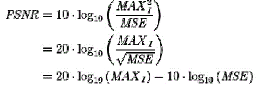
| Often abbreviated PSNR is an engineering term for the ratio between the maximum possible power of a signal and the power of corrupting noise that affects the fidelity of its representation. Because many signals have a very wide dynamic range, PSNR is usually expressed in terms of the logarithmic decibel scale. The PSNR (in dB) is defined as: |
 |
RESULT AND DISCUSSION
|
| Using Spatial Median Filter and Mean Filter we can reconstructed noise image as shown in below figures. By using mean filter total noise not reduced but median filters using total noise reduced as shown below figures. |
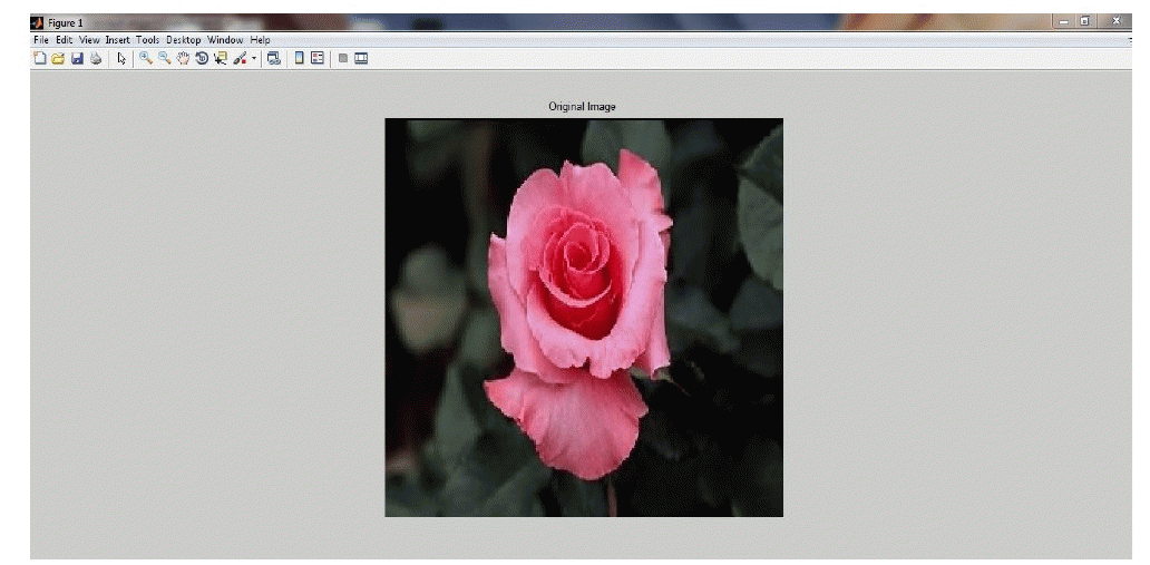
| In the fig 4, it shows the original image.here we are selecting the original image for adding noise in next stages. |
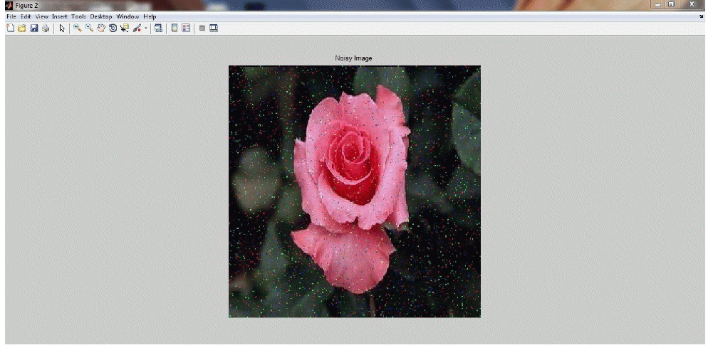
| In the fig 5, it shows the noise image. Here we are adding noise to original image by selecting the droupdown list in that list consist the levals of the noises. By selecting the noise leval we can apply the noise to the orinal image in matlap software by using GUI application. |
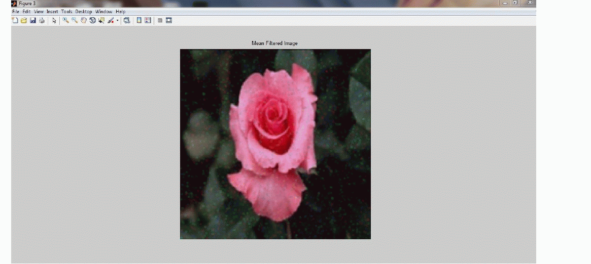
| In the fig 6, it shows we are applying the mean filter to the noise image then the noise images some noise are reduced. But the total noise is not reduced by using mean filter. |
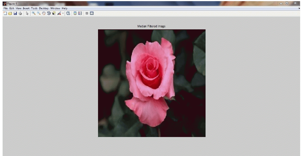
| In the fig 7, it shows the median filter output image. We are applying the median filter to the noise image then the noise of that image totally reduced. |
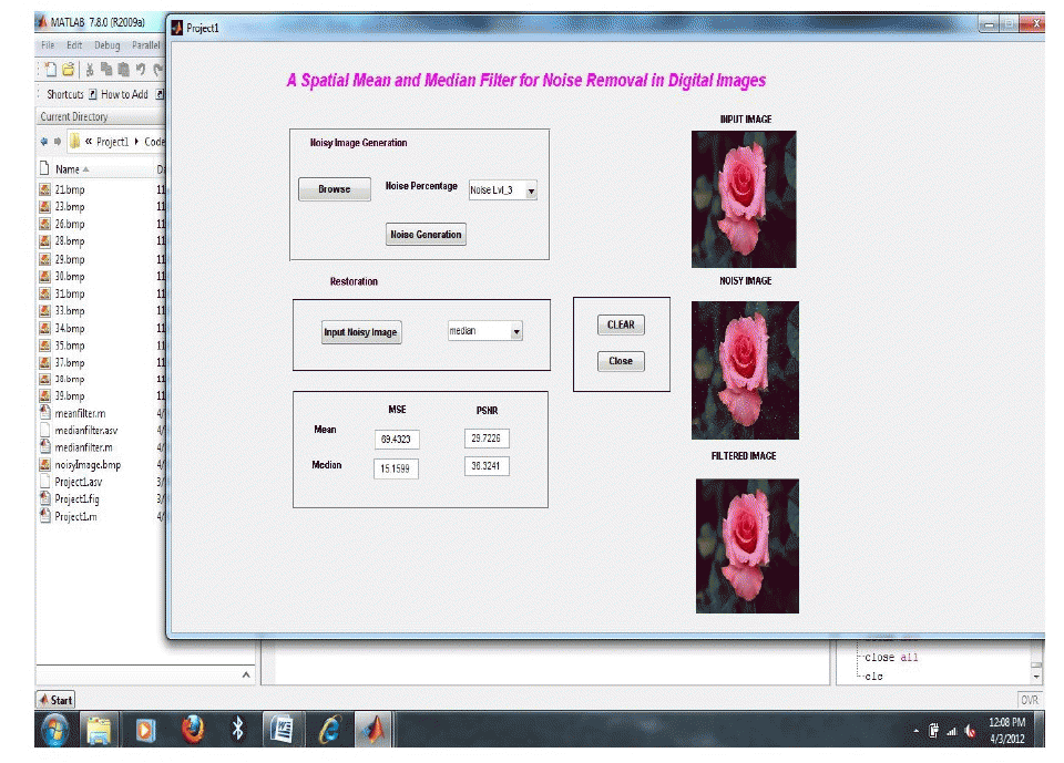
| In the fig 8, it shows the MSE and PSNR values for mean and median filters applied images. From those value we can identified more quality image. |
CONCLUSION
|
| We have introduced two filters for removing impulse noise from images. The Median filter outperforms the Mean filter as it does not make many changes to the uncorrupted pixel. In this comparison of noise removal filters, the experiment has been conducted for different images and at various noise levels, and is seen that Median filters performed the best overall noise compositions tested by providing minimum MSE. |
Figures at a glance
|
 |
 |
 |
 |
| Figure 1 |
Figure 2 |
Figure 3 |
Figure 4 |
 |
 |
 |
 |
| Figure 5 |
Figure 6 |
Figure 7 |
Figure 8 |
|
| |
References
|
- J. W. Tukey, ‘Nonlinear (Nonsuperposable)’, Methods for Smoothing Data. Conference Record EASCON, pp. 673-685, 1974.
- N. C. Gallagher, Jr. and G. L. Wise, A Theoretical Analysis of the Properties of Median Filters. IEEE Transactions on Acoustics, Speech, andSignal Processing, Vol. 29, pp. 1136-1141, 1981.
- JaakkoAstola, Petri Haavisto, and Yrj¨oNeuvo, Vector Median Filters.Proceedings of the IEEE, Vol. 78, No. 4, pp. 678-689, 1990.
- ProbalChaudhuri,On a Geometric Notion of Quantiles for Multivariate Data. Journal of the American Statistical Association, Vol. 91, No. 434,pp. 862-872, 1996.
- Robert Serfling,A Depth Function and a Scale Curve Based on Spatial Quantiles. In Y. Dodge (Ed.): Statistical Data Analysis Based on the L1-Norm and Related Methods Published by Birkh¨auser Basel, pp. 25-38, 2002.
- Yehuda Vardi and Cun-Hui Zhang, The Multivariate L1-median and Associated Data Depth.Proceedings of the National Academy of Sciences, Vol. 97, No.4, pp. 1423-1426, 2000.
|