Index Terms
|
| Query Processing, Spatial keyword queries, Spatial Database and Textual Database |
INTRODUCTION
|
| The range of technologies combines to afford the web and its users a geographical dimension. Geo-positioning technologies such as GPS and Wi-Fi and cellular geo-location services, e.g., as offered by Skyhook, Google, yahoo and Spotigo, are being used increasingly; and different geo-coding technologies enable the tagging of web content with positions. The percentage is likely to be higher for mobile users. This renders so-called spatial keyword queries important. Such queries take a location and a set of keywords as Arguments and return the content that best matches these arguments. The Google Maps and a yellow pages are the best Examples for providing a local search service in spatial keyword queries, where they enable search for, e.g., restaurants annotated with a text), a query location (latitude and longitude), and a set of querykeywords, a top-k spatial keyword query on road networks returns the k best objects in terms of both 1) shortest path to the query location, and 2) textual relevance to the query keywords. |
| For example, Figure 1 illustrates the road networks and spatial textual objects in a tourist area of Norway. The circles represent spatial-textual objects p with a textual description, and the cross mark q.l represents the query location. Assume a tourist in q.l with a GPS-enabled mobile phone. The tourist poses a top-kspatial keyword query looking for “hotel” (his spatial location is automatically sent by the mobile phone). If a traditional query (Euclidean distance) is considered, the top- 1 hotel is p9 on the left sideof the figure. However, when road networks are considered, the top-1 hotel is p4 on the right side of the figure. In top-k spatial keyword queries on road networks both shortest path and textual relevance are considered. For example, for the query “bar café” posed in q.l, the spatial-textual object p6 may appear better ranked than p7 because the description of p6 (“Egon Solsiden bar & café”) is more textually relevant to the query keywords than the descriptionof p7 (“Choco café”), and p6 is only slightly more distant to q.l than p7. The top-1 object, however, is p10 because it is very near to q.l and is also relevant to the query keywords. Note that p11 is not returned as a result of this query, since none of the terms in thedescription of p11 appear in the query keywords. The joint processing is motivated by main applications.a. Multiple Query Optimizations and b. Privacy-Aware Querying Support. |
NOVEL ALGORITHMS
|
| The existing IR-tree and then proceed to develop a basic and an advanced algorithm,for processing joint top k spatial keyword queries. The algorithms are generic and are not tied to a particular index. |
2.1 IR-Tree
|
| The IR-tree [2], which we use as a baseline, is essentially an R-tree [5] extended with inverted files [32]. The IR-tree’s leaf nodes contain entries of the form (p, p.λ, p.di), where p refersto an object in dataset D, p.λis the bounding rectangle of p,andp.diis the identifier of the description of p. Each leaf node also contains a pointer to an inverted file with the textdescriptions of the objects stored in the node. An inverted file index has two main components. |
| • A vocabulary of all distinct words appearing in the description of an object. |
| • A posting list for each word t that is a sequence of identifiers oftheobjects whose descriptions contain t. |
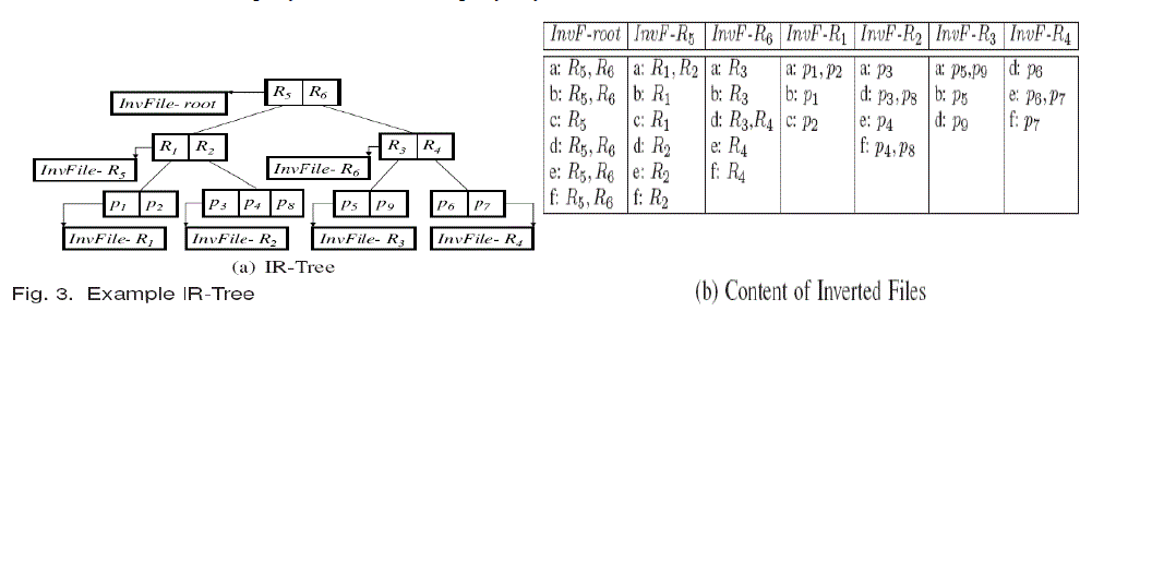
| Each non-leaf node R in the IR-tree contains a number of entries of the form (cp, rect, cp.di) where cpis the address of a child node of R, rectis the MBR of all rectangles in entries of the child node, and cp.diis the identifier of a pseudo text description that is the union of all textdescriptions in the entries of the child node. As an example, Figure 2a contains 8 spatial objects p1, p2, . . . , p8, and Figure 2b shows the words appearing in the description of each object. Figure 3a illustrates the corresponding IR-tree, and Figure 3b shows the contents of the inverted files associated with the nodes. |
2.2 LOOPING Algorithm and JOINT Algorithms
|
| The LOOPING algorithm for computing the joint top-k spatial keyword query isadapted from an existing algorithm [2] that considers a single query. Recall that a joint top-k spatial keyword query Q consists of a set of sub queries qi. The LOOPING algorithm computes the top-k results for each sub query separately. The arguments are a joint query Q, the root of an index root, and the number of results k for each sub query. When processing a sub query qi ∈Q, the algorithm maintains a priority queue U on the nodes to be visited. The key of an element e ∈U is the minimum distance mindist(qi.λ, e.λ) between the query qi and the element e. The algorithm utilizes the keyword information to prune the search space. It only loads the posting lists of the words in qi. A non-leaf entry is algorithm returns k elements that have the smallest Euclidean distance to the query and contain the query keywords. |
| Example 1: Consider the joint query Q = {q1, q2, q3} in Figure 2, where q1.ψ = {a, b}, q2.ψ = {b, c}, q3.ψ = {a, c},and all sub queries (and Q) have the same location λ. Table 1shows the minimum distances between Q and each object and bounding rectangle in the tree. We want to find the top-1 object. For each sub query qi, LOOPING thus computes the top-1 result. Subqueryq1 =_λ, {a, b}_first visits the root and loads the posting lists of words a and b in InvFile-root. Since entries R5 and R6 both contain a andb, both entries are inserted into the priority queue with their distances to q1. The next dequeued entry is R5, and the posting lists of words a andb in InvFile-R5 are loaded. Since only R1 contains a andb, R1 is inserted into the queue, while R2 is pruned.NowR6 and R1 are in the queue, and R6 is dequeued. After loading the posting lists of words a andb in InvFile-R6, R3is inserted into the queue, while R4 is pruned. Now R1 andR3 are in the queue, and R1 is dequeued. Its child node is loaded, and the top-1 object p1 is found, since the distance of p1 is smaller than that of the first entry (R3) in the queue(2 <4). Similarly, the result of sub query_λ, {b, c}_is empty and the result of sub query is λ, {a, c}is P2. The dis advantage of theLOOPING Algorithm is that it may visit a tree node multiple times, leading to high I/O cost. |
| The JOINT Algorithm: The JOINT algorithm aims to process all sub queries of Q concurrently by employing a shared priority queue U to organize the visits to the tree nodes that can contribute to closer results (for some sub query). Unlike LOOPING, JOINT guarantees that each node in the tree is accessed at most once during query processing. |
| Pruning Strategies: The algorithm uses three pruning rules. Let ebe an entry in a non-leaf tree node. We utilize the MBR and keyword set of e to decide whether its sub tree may contain only objects that are farther from or irrelevant to all sub queries of Q. |
| ? Cardinality-Based Pruning |
| ? MBR-Based Pruning |
| ? Individual Pruning. |
NOVEL INDEXES AND ADAPTATIONS
|
| We present the TB-IR-tree that organizes data objects according to both location and keywords. We discuss the processing of the jointtop-k query using existing indexes. |
3.1 The Text based-IR-Tree (TBIR TREE)
|
| Text Based Partitioning: As a first step in presenting the index structure, we consider the partitioning of a dataset according to keywords. We hypothesize that a keyword query will often contain a frequent word (say w). This inspires us to partition dataset D into the subset D+ whose objects contain w and the subset D−whose objects do not contain w and that we need not examine whenprocessing a query containing w. We aim at partitioning D into multiple groups of objects, such that the groups share as few keywords as possible. However, this problem is equivalent to, e.g., the clustering problem and is NPhard. Hence, we propose a heuristic to partition the objects.Let the list W of keywords of objects sorted in descending order of their frequencies be: w1, w2, . . . ,wm, where m is the number of words in D. Frequent words are handled before infrequent words. We start by partitioning the objects into two groups using word w1: the group whose objects contain w1,and the group whose objects do not. We then partition each of these two groups by word w2. This way, the dataset can be partitioned into at most 2, 4, . . . ,2m groups. By construction, the word overlap among groups is small, which will tend to reduce the number of groups accessed when processing a query. Algorithm 3 recursively applies the above partitioning to construct a list of tree nodes L. To avoid underflow and overflow, each node in L must contain between B/2 and B objects, where B is the node capacity. In the algorithm, D isthe dataset being examined, and W is the corresponding wordlist sorted in the descending order of frequency. When the number of objects in D (i.e., |D|) is between B/2and B, D is added as a node to the result list L (lines 1–2).If |D| < B/2 then D is returned to the parent algorithm call(lines 3–4) for further processing. If |D| > B (line 5) then we partition D (lines 6–19).In case W is empty (line 6), all the objects in D must have the same set of words and cannot be partitioned further by words. We hence use a main-memory R-tree with fan out(node capacity) B to partition D according to location and add the leaf nodes of the R-tree to the result list L (lines 7–8).When W is non-empty, we take the most frequent (first)word in W (lines 9–10). The objects in D are partitioned into groups D+ and D−based on whether or not they contain w (lines 11–12). Next, we recursively partition D+ and D−(lines 13–14). The remaining objects from these recursive calls (i.e., the sets T+ and T−) are then merged into the set T_(line 15). If T_ has enough objects, it is added as a node to L (lines 16–17). Otherwise, set T_ is returned to the parent algorithm call (lines 18–19).If the initial call of the algorithm returns a group with less than B/2 objects, it is added as a node to the result list L, since no more objects are left to be merged. |
| Algorithm The TBIR TREE Dataset D, Sorted list of words W, Integer B, List of tree nodes L |
| 1: if B/2 ≤ |D| ≤ B then |
| 2: add D as a node to L; |
| 3: else if |D| < B/2 then |
| 4: return D; |
| 5: else _ partitioning phase |
| 6: if W is empty then _ partitioning by location |
| 7: insert D into a main-memory R-tree with fanoutB; |
| |
| 8: add the leaf nodes of the main-memory R-tree to L; |
| 9: else _ partitioning by words |
| 10: w ← first word in W; W ← W \ {w}; |
| 11: D+ ← {p ∈ D | w ∈p.ψ}; |
| 12: D− ← {p ∈ D | w /∈p.ψ}; |
| 13: T+ ← WordPartition(D+,W,B, L); |
| 14: T− ← WordPartition(D−,W,B, L); |
| 15: T_ ← T+ ∪ T−; |
| 16: if B/2 ≤ |T_| ≤ B then |
| 17: add T_ as a node to L; |
| 18: else if |T_| < B/2 then |
| 19: return T_; |
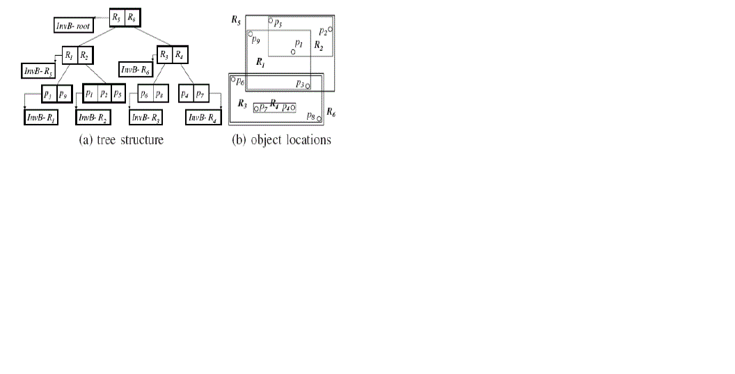
| Tree Construction Using TBIR TREE:The TBIR TREEuses the same data structures as the IR-tree, but is constructed differently by using Text based partitioning (thus the prefix ‘W’). Instead of performing insertions iteratively, we build the TBIR TREE-tree bottom-up. We first use the TBIR TREE partitioning (Algorithm 3) to obtain the groups that will form the leaf nodes of the TBIR TREE-tree. For each leaf node N, we compute N.ψas the union of the words of the objects in node N, and N.λas the MBR of the objects in N. Next, we regard the leaf nodes as objects and apply Algorithm 3 to partition the leaf nodes into groups that form the nodes at the next level in the TBIR TREE. We repeat this process until a single TBIR TREE root node is obtained. Figure 4a illustrates the TBIR TREEfor the 8 objects in Figure 4b. Following Example 3, leaf nodes R1 ← {p3, p9}, R2 ← {p1, p2, p5}, R3 ← {p6, p8}, and R4 ← {p4, p7} arefirst formed. Figure 4b shows the MBRs of those leaf nodes and R1.ψ = {a, d}, R2.ψ = {a, b, c}, R3.ψ = {d, e, f},R4.ψ= {e, f}. Next, Algorithm 3 is used to partition R1,R2, R3, and R4, since they are 4 (the node capacity is 3)nodes and cannot be put into one node at the next level. Using7word a, two partitions are obtained, i.e., R5 ← {R1,R2} andR6 ← {R3,R4}. Since R5 and R6 contain between 1.5 and 3nodes, there is no need to further partition them. Finally, R5and R6 can be put into one node at the next level, resulting the root node of the TBIR TREE. |
| The IR-tree and the TBIR TREEorganize the data objects differently. The IR-tree organizes the objects purely based on their spatial locations. In contrast, the TBIR TREEfirst partitions the data objects based on their keywords (Lines 10–19) and then further partitions them based on their spatial locations(Lines 6–8). Thus, the TBIR TREE-tree matches better the semantics of the top-k spatial keyword query and have the potential to perform better than the IR-tree. |
| Updates:A deletion in the TBIR TREEis done as in the R-tree, by finding the leaf node containing the object and then removing the object. An insertion selects a branch such that the insertion of the object leads to the smallest “enlargement” of the keyword set, meaning that the number of distinct words included in the branch increases the least if the object is inserted there. |
3.2 The TB-IBR-Tree and Variants
|
| Inverted Bitmap Optimization:Each node in the TBIR TREE contains a pointer to its corresponding inverted file. By replacing each such inverted file by an inverted bitmap, we can reduce the storage space of the TBIR TREEand also save I/O during query processing. We call the resulting tree the TB-IBR-tree. |
| IBR-Tree and CD-IBR-Tree: The inverted bitmap optimization technique is applicable to the original IR-tree [2], yielding the IBR-tree. The bitmap optimization technique is also applicable to the CDIR-tree [2], yielding the CD-IBR-tree. |
3.3 Query Processing Using Other Indexes
|
| The LOOPING AND JOINT algorithms are generic and are readily applicable to the proposed indexes, including the TBIR-tree and the TB-IBR-tree; the existing indexes, e.g., the IR treeand the CDIR-tree; and the existing indexes using the optimizations proposed in this paper, including the IBR-tree and CD-IBR-tree |
I/O COST MODELS FOR THE IR-TREE ANDTHE TBIR TREE
|
| A cost model for an index is affected by how the objects are organized in the index. The Inverted-R-trees, the IR2-tree, the IR-tree, and the IBR-tree adopt spatial proximity, as does theR-tree, to group objects into nodes. The TBIR TREE and the TB-IBR-tree use word partitioning to organize objects. This section develops an I/O cost model for each of the IR-tree and the TB-IR-tree that then serve as representatives of the above two index families. The cost model of the CD-IBR-tree is inbetween those of the two families, since it considers both spatial proximity and text relevancy .Specifically, the models aims to capture the number of leaf node accesses, assuming that the memory buffer is large enough for the caching of nonleaf nodes.2 We also ignore the I/O cost of accessing posting lists as this cost is proportional to the I/O cost of accessing the tree. The resulting models provide insight into the performance of the indexes.Like previous work on R-tree cost modeling [24], we make certain assumptions to render the cost models tractable. We assume that the locations of objects and queries are uniformlydistributed in the unit square [0, 1]2. Let n be the number of objects in the dataset D, and let B be the average capacity of a tree node. Thus, the number of leaf nodes is NL = n/B. We assume that the frequency of keywords in the dataset follows a Zipfian distribution [16], [31], which is commonly observed from the words contained in documents. Let the word wibe the i-th most frequent word in the dataset. The occurrence probability of wiis then defined as |
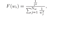 |
| where Nwis the total number of words and s is the value of the exponent characterizing the distribution (skew).Let a query be q = _λ, ψ_. Suppose that each object and the query contain z keywords. We assume that the words of each object are drawn without replacement based on the occurrence probabilities of the words. Let dknndenote the kNN distance of q, i.e., the distance to the kthnearest neighbor in D. Let ebe any non-leaf entry that points to a leaf node. We need to access e’s leaf node when: |
| 1) the keyword set of e contains q.ψ, and |
| 2) the minimum distance from q to e is within dknn. Let the probability of the above two events be the keywordcontainment probability Pr(e.ψ⊇q.ψ) and the spatial intersectionprobability Pr(mindist(q, e.λ) ≤ dknn), respectively. Thus, the access probability of the child node of e |
| is:Pr(access e) = Pr(e.ψ⊇q.ψ) · Pr(mindist(q, e.λ) ≤ dknn). |
| Estimate the total number of accessed leaf nodes as:COST = NL · Pr(access e) |
| We proceed to derive the probability of an object matching the query keywords and the kNN distance dknn. We then study the probabilities Pr(e.ψ⊇q.ψ) and Pr(mindist(q, e.λ) ≤ dknn) for the IR-tree and the W-IR-tree, respectively. Finally, we compare the two trees using the cost models. |
4.1 Estimation of Keyword Probability and kNN Distance
|
| Probability of an Object Matching the Query Keywords: |
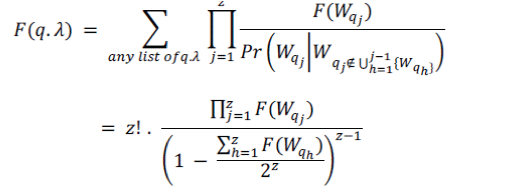
| Let F(q.λ) be the probability of having q.λas the keyword set of an object of D. Let z be the number of words in each object (and also in the query). Let an arbitrary list (i.e., sequence) of q.λbe wq1, wq2 ,· · · , wqz. Due to the “without treplacement” rule, when we draw the j-th word of an object, any previously drawn word (wq1, wq2 ,· · · , wqj−1 ) cannot be drawn again. Thus, the probability of the j-th drawn word being wqjis: |
 |
| The probability of drawing the exact list wq1,wq2 , · · ,wqzis: |
 |
| sum up the probability for every list enumeration of q.λ. As there are z! such lists, the probability of having q.λas the keyword set of an object p ∈ D is: |
 |
| kNN Distance:Observe that the kNN distance dknnof q depends only on the dataset D, but is independent of the tree structure. The number of objects having the keyword q.ψis: n · F(q.ψ). By substituting this quantity into the estimation model of Tao et al. [23], we estimate the kNN distance of q as |
 |
| We then approximate the kNN circular region _(q, dknn)by a square having the same area, i.e., with the side-length l = √π·dknn. According to Theodoridis et al. [24], the spatial intersection probability is: |
| Pr(mindist(q, e.λ) ≤ dknn) ≈ (σ + l)2 = (σ + √π · dknn)2, |
| whereσ is the side-length of non-leaf entry e. We shortly provide detailed estimates of σ for both trees. |
4.2 I/O Cost Models
|
| IR-Tree: The construction of the IR-tree proceeds as for the R-tree [33] .Objects are partitioned into leaf nodes based on their spatial l proximity. We consider the standard scenario where the leaf nodes are squares and form a disjoint partitioning of the unit square. Therefore, we have NL · σ2ir= 1, and we then obtain σir= _1/NL. The spatial intersection probability is derived by substituting σirinto Equation 3.Given the query keyword q.ψ, the keyword set of e contains q.ψif some object (in the child node) of e has the keyword q.ψ. Note that in the IR-tree, the keywords of the objectsin the leaf node pointed to by eare distributed randomly and independently. Since the leaf node has capacity B, the keyword containment probability is |
| Prir(e.ψ⊇w) = 1 − (1 − F(q.ψ))B. |
| TBIR-TREE: During the construction of the TB-IR-tree, the objects are first partitioned based on their keywords. Thus, the number of leaf nodes that contain the query word q.ψis: max{NL · F(q.ψ), 1}. Then the objects in these nodes are further partitioned into nodes based on their locations. By replacing NL with max{NL · F(q.ψ), 1} in Equation 3, we obtain |
| σtbir= _1/ max{NL · F(q.ψ), 1}. (4) |
| We obtain the spatial intersection probability by substituting σtbirinto Equation 3.Observe that out of NL leaf nodes, max{NL · F(q.ψ), 1} nodes contain the query keyword q.ψ. Thus, the keyword containment probability is |
 |
CONCLUSION AND FUTURE ENHANCEMENT
|
| The joint top-k spatial keyword query and presents efficient means of computing the query. Our solution consists of: (i) the TB-IBR-tree that exploits keyword partitioning and inverted bitmaps for indexing spatial keyword data, and (ii) the JOINT algorithm that processes multiple queries jointly. In addition, we describe how to adapt the solution to existing index structures for spatial keyword data. Studies with combinations of two algorithms and a range of indexes demonstrate that the JOINT algorithm on the TB-IBR-tree is the most efficient combination for processing joint top-k spatial keyword queries. It is straightforward to extend our solution to process top-k spatial keyword queries in spatial networks. We take advantage of Euclidean distance being a lower bound on network distance. While reporting the top-k objects incrementally, if the current object is farther away from the query in terms of Euclidean distance than is the kthcandidate object in terms of network distance, the algorithm stops and the top-k result objects in the spatial network are found. The network distance from each object to a query can be easily computed using an existing, efficient approach [20].An interesting research direction is to study the processing of joint moving user. |
Figures at a glance
|
 |
 |
 |
 |
| Figure 1 |
Figure 2 |
Figure 3 |
Figure 4 |
|
References
|
- X. Cao, G. Cong, C. S. Jensen, and B. C. Ooi.Collective spatialkeyword querying.In SIGMOD, 2011.
- R. Hariharan, C. Li, and S. Mehrotra. Processing spatial-keyword (SK) queries in In SSDBM, p. 16, 2007.
- H. Hu, J. Xu, and W. C Lee. Proactive caching for spatial queries in mobile environments., pp. 403–414, 2005.
- H. Lu,. PAD: privacy-area aware, dummy-based location privacy in mobile Services. In MobiDE, pp. 16–23, 2008.
- B. Martins, M. J. Silva, and L. Andrade. Indexing and ranking in geo-IR systems. In GIR, pp. 31–34, 2005.
- M. Murugesan and C. Clifton.Providing privacy through plausibly deniable search.In SDM, pp. 768–779, 2009.
- H. Samet, and H. Alborzi. Scalable network distance browsing in spatial databases. In SIGMOD,pp. 43–54, 2008.
- T. K. Sellis. Multiple-query optimization.IEEE TKDE, 16(10):1169–1184, 2004.
- D. Zhang Keyword search in spatial databases: towards searching by document. In ICDE, pp. 688–699, 2009.
- D. Zhang, B. C. Ooi, and A. Tung. Locating mapped resources in web 2.0.In ICDE, pp. 521–532, 2010.
- J. M. Edgington, STR: A simple and efficient algorithm for R-tree packing. In ICDE,pp. 497–506, 1997
- B. Zheng and D. L. Lee.Semantic Caching in Location-Dependent Query Processing.In SSTD, pp. 97–116, 2001.
- Y. Zhou,. Hybrid index structures for location-based web search. In CIKM, pp. 155–162, 2005.
- G. K. Zipf. The Psycho-Biology of Language.Houghton Mifflin, Boston, 1935.
- J. Zobel and A. Moffat. Inverted files for text search engines. ACM Comput.Surv., 38(2):6, 2006.
- M. Hong, Rule-based multi-query optimization. In EDBT, pp. 120–131,2009.
- L. Kaufman Finding groups in data: anintroduction to cluster analysis. New York: Wiley, 1990.
- H. Kido,An anonymouscommunication technique using dummies for location-based services.In IEEE conf. on pervasive Services,pp. 88-97,2005.
- L. Kulik. A formal model of obfuscation andnegotiation for location privacy. In PERVASIVE, pp. 152–170,2005.
- D. Wu. Efficient retrieval of the top-k most relevant spatial web objects. In VLDB,pp. 337–348,200
|