ISSN: 2320-2459
ISSN: 2320-2459
Das RK*
Physics and Applied Mathematics Unit, Indian Statistical Institute, Kolkata, India
Received date: 20/07/2021; Accepted date: 16/08/2021; Published date: 26/08/2021
Visit for more related articles at Research & Reviews: Journal of Pure and Applied Physics
LTB metric (Lemaître-Tolman-Bondi metric) is a spherically symmetric dust solution (zero pressure contribution in energy-momentum tensor) of Einstein field equation, basically which roles as one of the models of explanation about accelerating expansion of the universe. From the analytical treatment, the cosmic scale factor has been deduced from the framework of commoving coordinate system. Then a statistical approach of relative entropy has been drawn as the final result for three types of the universe (based on curvature: positive, flat, and negative).
Tensor analysis (algebra and calculus), General relativity, Einstein field equation, Basic theory of cosmology, Laws of thermodynamics.
Expanding universe is an important topic in modern cosmology. Expanding universe means to say the increase of distance between two points in space in the universe with time. After the big bang, the universe is suddenly expanding with time. When Einstein was developing the theory of general relativity [1,2], he predicted that if gravity is the only active interaction in the universe so by his theory universe should collapse. But at that time according to the astronomers, the universe was static, so Einstein introduced a constant to balance his equation for modelling a static universe; it is a cosmological constant [3]. Now later in 1929, Edwin Hubble showed by telescope observation data of redshift-distance relationship that the universe is expanding [4,5]. So this indicates there is no need for cosmological constant further and also by LTB metric [5,6] approach without considering the cosmological constant, it can be shown that universe is expanding. But for modern cosmological view the cosmological constant has an importance that is related to vacuum energy and it is useful to explain the dark energy concept of expanding universe (which is not our business for this moment). LTB model [6,7] is the good choice for this analysis of connection between relative entropy [8-10] and cosmic scale factor (which deals as a useful parameter to describe accelerated universe expansion).
Lemaitre-Tolman-Bondi metric is based upon the concept of commoving coordinate system. So this approach of commoving coordinate system is essential for easy calculations and a better understanding of universe expansion. Georges Lemaitre, Richard Tolman and Hermann Bondi made a framework on that Metric to understand the expanding universe model in 1934. The metric [6,7] is such that,

Φ(r,t) is the area distance function and Φ’(r,t) is the space derivative and k(r) is the curvature function and k(r)<1 here assuming. So next we have to further work out that metric.
We have to do now the mathematical investigation of LTB Metric through the gravitational field equation. So we see the form of Metric, which is kind of (-,+,+,+). So for this case corresponding field equation [1,2] will be such that,

Now we will be focus to deduce the required field equations according to the grammar of general relativity. More specifically we will be concern to cross-check the technical terms like Christoffel symbols and corresponding Ricci tensors by the equations

And observing the corresponding metric tensor ( gμϑ ) and energy-momentum tensor (Tμϑ )
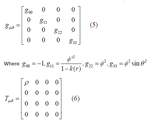
For this metric and corresponding energy-momentum tensor, we will get four field equations as a result
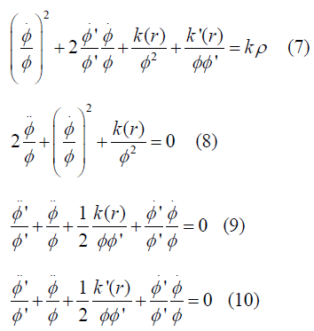
So now from 2nd field equation (8) we will get
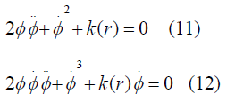

So finally it will be

Where M(r) is an arbitrary function chosen as time-independent integration constant Now From equations (7) and (9) we get
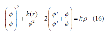
And using equation 11 and 14 we get

Now these two equations give
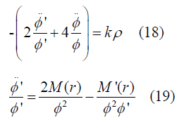
Finally, we have

Now we have to solve the equation (11) with three conditions of Curvature function k(r)=0, and k(r)>0, k(r)<0.
Case 1
K(r)=0 (Flat): So equation (14) stands for

With help of equation (11) we can write equation again

From that we can achieve that
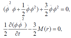
Now we will get a solution

At primary condition for the time ‘t’ such that
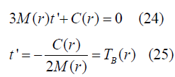
TB(r) (Big-bang time function)
Further solving we will get a solution [6,7]

Case 2
K(r) ≠ 0: Now for other cases we have got solution by Mathematica coding by parametric solution study such that (��(��,��) parametric function)[6,8].
K(r)>0 (positively curved): Solution is


K(r)<0 (negatively curved): Solution will be


According to FRW limit Ф=ra(t) and K(r)=((Const).r2) and we consider an assumption (“Const” denotes constant in equations) [9].

Where a(t) is the cosmic scale factor and for physical importance M(r)function roles as the mass of a commoving shell (minimal LTB void model) [9].
We will now do the part of the connection to statistical physics part so we have the results of general relativistic calculations on cosmological domain now we have to include the information theory in statistical physics, so now in the statistical physics domain if we have two kinds of probability distribution qi and pi where 2nd is actual distribution so we have to understand the distinguishability between them and also mutual information. We have to link an entropy for that goal, that is relative entropy [3,8].

So by the same analogy, we can also link an entropy means relative entropy that represents the measure of distinguishability between actual matter density and average matter density and mutual information so the relative entropy in unit volume [3,8].

Now we the special average of density in the commoving domain is defined as [8,10].

So from equation (20) applying FRW limit, we will get (here we only are focusing on time and we are treating radial part (related to spherical coordinate r) as constant.


Here gii is the metric tensor associated LTB Metric (excluding time part)
Using these we have achieved

And the relative entropy,

And final result
s = Rln a(t) − D (36) , where R and D are constant.
We previously have taken the assumptions and some modelling

So the cosmic scale factor as a solution based on the above assumptions
K(r)=0 (Flat, zero curvature):

K(r)>0 (positively curved): (A and B are constants)
a(t) = A(1− cosη ) (38)
(t) = B(η − sinη ) (39)
K(r)<0 (negatively curved): (E and F are constants)
a(t) = E(coshη −1) (40)
(t) = F(sinhη −η ) (41)
For zero curvature case, relative entropy can be easily determined
S = 2 / 3Rln t − D (42) ,
where R and D are the same constants which are used also in equation (36).
Now if we try to plot the relative entropy with time, we will get the result shown in Figure 1.
Now for positively and negatively curved cases, it is too hard to determine the exact nature, so here we will use the Mathematica technique to plot parametric equations and to observe the nature of relative entropy.
According to this, the obtained result is shown in Figure 2.
So from this investigation, we have seen such that relative entropy for flat universe case increases with time and the almost same result for negative curvature. But for positive curvature cases (Figure 3) at certain times relative entropy is falling down, according to physics or thermodynamics which is not a well-defined phenomenon. For any kind of physical phenomena, associated entropy should increase. Actually, this result supports the overall spatial flatness of the universe. The contribution of curvature is very small; our universe is almost spatially flat.
I am sincerely thankful to Dr Ajay D. Thakur Associate Professor, Department of Physics, Indian Institute of Technology Patna, (Bihar, India) who was my master project supervisor during my MSc. period. He always has motivated me for my work. I am also thankful to Department of Physics (IITP) to give me an opportunity to work on this project. As an overall result today I have been able to make some outcome for this manuscript.