Bayesian Hierarchical Functional Data Analysis for Healthy Menstrual Cycles

Abstract

In almost every field of study, studying the distribution of a random curve can give needed information. In the field of in vitro fertilization, particular interest is given to modeling the temperature curves of women across their menstrual cycle. Fitting the curve can lead to categorizing cycles as healthy or unhealthy and can help identify the most fertile days of a cycle.

Keywords

Hierarchical model, Gibbs sampling, Simulation, Bayesian specification, Menstrual cycles.

Introduction

In almost every field of study, studying the distribution of a random curve can give needed information. In the field of in vitro fertilization, particular interest is given to modeling the temperature curves of women across their menstrual cycle. Fitting the curve can lead to categorizing cycles as healthy or unhealthy and can help identify the most fertile days of a cycle. A healthy menstrual cycle consists of three phases, the follicular phase, ovulation, and the luteal phase. During the follicular phase, the basal body temperature (the lowest temperature reached during rest, referred to as bbt for the remainder of this paper) holds constant at a low plateau. During ovulation, the bbt increases until it hits the high plateau. The bbt then holds constant at this high plateau through the luteal phase. At the end of the cycle, the bbt drops back down to the low plateau before menstruation and the cycle repeats [1]. Figure 1 gives a few examples of a healthy menstrual cycle’s bbt levels [2]. Section 2 outlines the general hierarchical model, then gives a parametric modeling of the bbt curves. The end of Section 2 completes the Bayesian specification and specifies the hyperparameters needed for the prior distributions. Section 3 briefly describes how the Gibbs sampling algorithm works and then applies it to model. Section 4 gives a short description of the change-point problem and defines the stopping rule needed in order to identify the two change-points in the model. Section 5 details a simulation of the data and then applies the Gibbs sampling algorithm with intentionally skewed hyperparameters. The results of the simulation are discussed at the end of Section 5. Finally, Section 6 provides a short discussion of the model and conclusions.

The Hierarchical Model

First, we will define terms necessary to describing the model. A prior distribution of an unknown quantity X is the probability distribution that would express one’s certainty about X before the data is taken into account. Similarly, a posterior distribution of an unknown quantity X is the probability distribution of that quantity conditional on the observed data. A hyperparameter is parameter of a prior distribution that is not treated as random. For example, consider a random variable X that came from A distribution, where Σ is known and we can use a distribution to model μ. Then μ is a parameter, is a prior distribution, and μ₀ and Σ₀ are hyperparameters.

The General Model

Let refer to woman i,jε {1,2,.....n_i} refer to cycle j of woman i, and refer to day t in cycle j of woman i. These indices will retain these definitions throughout the remainder of the paper. We can establish the following model for bbt curves [3]:

where ε_ij is the measurement error and η_ij is a smooth function from to .Since cycles of the same woman are expected to be correlated, we can establish a prior distribution for the distribution of functions for woman call it G_i . However, healthy menstrual cycles will follow a similar pattern among women, so we can establish a prior distribution for the collection of distributions for the different women , call it P. Thus if we assume our error is normally distributed, we have the following model [3]:

Basis representation

Now that we have our general model, there are a number of different representations that could be used for η_ij. A common strategy is to consider a basis representation [3]:

where are pre-specified basis functions and are cycle-specific basis coefficients. Since is prespecified, our major objective is to model the θ_ijs. The approach we use is to give the θ_ijs a hierarchical normal model [3]:

Where N_k(μ,Σ) is the multivariate normal distribution with mean vector μ and covariance matrix Σ. The woman-specific basis coefficients are given by αi, α gives the global mean basis coefficients, and Ω and Ω₁ are the precision matrices for the within and between woman variability respectively. So to complete the model, we need to specify the basis functions and establish the components of θ_ij. We’ll do this in the next section when we consider a parametric hierarchical structure.

Parametric Hierarchical Model

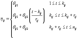
As we discussed in Section 1, bbt levels of a healthy cycle follow a biphasic pattern where the bbt levels start at the low plateau in the follicular phase then quickly rise during ovulation to the high plateau in the luteal phase. Thus we can model η_ij (t) as follows [3]:

where where θ_ij1 and θ_ij2 indicate the temperature during the follicular phase and the increase in bbt during ovulation respectively for cycle j of woman i. We can further define to be the last day of the follicular phase and r_ij to be the number of days the bbt rises during ovulation (Figure 2). Thus, if we consider y_ij (t) as Y_ij a vector of n_ij bbt values, we can represent our hierarchical model in matrix form [3]:

Thus X_ij (t), the t^th row of X, corresponds to tth day of cycle j of woman i. So we have defined our pre-specified basis function and our cycle-specific basis coefficients .

Bayesian Specification

Now we have within (Ω) and between (Ω₁) woman variability, the last day of the follicular phase (k_ij), the number of days during ovulation (r_ij), the global mean (α), and measurement error variance (σ₂) left to model. We’ll use the following equations to model the within and between woman variability:

We complete the Bayesian specification with the following priors [3]:

where is the gamma distribution with shape parameter a and inverse scale parameter b, is the discrete uniform distribution between a and b, and mij is the first day after menstruation. Thus, our pre-specified hyperparameters are α₀, Σ_α, c, d, a_h, b_h, a_h1, and b_h2 (for h = 1, 2).A summary of the parameters, hyperparameters, their descriptions, and distributions is given in the appendix.

Gibbs Sampling

Our goal is to find the parameters of our model given a set of observations. Since finding the joint distribution is a complicated process, we need to use a different method. A common method to do this is to use a Monte Carlo Markov Chain as an iterative procedure. The specific type of Monte Carlo Markov Chain that we’ll use is called a Gibbs sampler.

Definition

Suppose we have random variables X₁, X ₂,…, X _n.

1. Initialization: Let be given some initial value.

2. Iteration: For 1 ≤ I≤ K, sample x _(i)^j from the conditional distribution of X_j given and for 1 ≤ j ≤ n

This Gibbs sampling procedure is a Markov chain, where the stationary distribution is joint distribution of X₁, X ₂,…, X _n.Thus, for large k, the sample approximates the joint distribution of X₁, X ₂,…, X _n. .A blocked Gibbs sampler uses the same steps, except it groups some of the random variables together so that the variables in a block are sampled from their joint distribution conditioned on all other variabes.

Gibbs Sampling Algorithm

Here is the blocked Gibbs sampling algorithm for our model after we’ve given the parameters some initial value [2]:

1. Cycle-specific coefficients:

2. Women-specific means:

3. Global mean:

4. Components of Ω( h = 1,2):

5. Components of

6. Error variance:

7. Last day of follicular phase: Use the change-point stopping rule for k_ij (see Section 4).

8. Ovulation period: Use the change-point stopping rule for r_ij (see Section 4).

So if we use the blocked Gibbs sampling steps to update the unknown parameters from their conditional distributions, then after a large number of iterations, we’ll be sampling from the joint distribution of all the unknown parameters.

Change-Point Problem

Now we need to consider kij and rij since these are specific points (called change-points) in the bbt curve where the shape of the curve changes. The process for finding a change-point P is intuitive. Given a set of observations .we’ll find the probability that p ≤ m given ym . We want this probability to be higher than some high threshold Q. Thus we have a “stopping rule" [4]:

Terminate at m if and only if

Starting with m = 1, the first time that the probability is greater than Q is our change-point P.

Finding kij

First we wish to find k_ij assuming that the other parameters are known. Let X_k be the first m rows of the matrix X_ij established above but with k_ij = k. Thus . Let {π_k} be the prior distribution for k_ij,π(.) be the density function of θ_ij, and f(.) be the density function of the data yij,m. We now need to find the posterior distribution of k_ij in order to find for our stopping rule.

Let be the change-point likelihood. Then implementing Bayes’ theorem, we get [4]

Since L_k is not a function θ_ij we may replace θ_ij with 0. Also does not depend on k, so L_k is proportional in k to

The posterior distribution of θ_ij is N₂(μ_k,V_k) where

Note that this is the same posterior distribution found for θ_ij found in Section 3, but with the altered matrix X_K . Using this posterior distribution for θ_ij , we find that

Since we need to find , we’ll first find .From applying Bayes’ theorem to , we get

Since L_K is proportional in k to W_K, then we can substitute Wk in for L_K , resulting in

These probabilities are easy to compute as the data becomes available. When k ≥ m,

So X_K does not depend on k (and hence W_K = W_M). Thus, our stopping rule is to terminate at m if and only if

Once we hit our stopping rule [4], let k_ij =m.

Finding r_ij

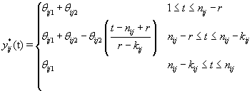
We can apply the same approach to finding r_ij by using a transformation to examine the data “backwards", i.e. consider the last day first, and proceed through the cycle in reverse order. So our new reversed data is

Let be our transformation matrix. Then

Thus if we let Xr* correspond to the first m rows of the above system, then

This transformation lets us use the same process that we used to find k_ij. Let {π_r } be the prior distribution for r (the second changepoint). The new posterior distribution for θ*_ij is N₂(μ_r,V_r), where

Note that since thus giving a similar posterior distribution found in Section 3 for θ_ij. Using this posterior distribution for *_ijwe find that

Thus, our stopping rule is to terminate at m if and only if

Once we hit our stopping rule, r =n_ij-m (since we transformed our data). Since r_ij is the number of days between k_ij and r, then r_ij = r –k_ij

Simulation

Data simulation

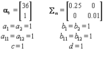
Now that the method has been described, we’ll introduce a simulation in order to illustrate the method. The simulated data consisted of 20 women, each with 10 cycles, so we had a total of 200 cycles. Each cycle had a length of 30 days [5]. We arbitrarily assigned the global mean and covariance matrices to be

Each woman specific mean was generated as per the model discussed in Section 2, so We then generated kij and rij for each cycle according to .Finally, we generated the cycle specific coefficients according to and the measurement error terms according to where σ ²= 0.01. Now that we generated all the parameters needed for our model, we generated the bbt values according to

Initialization

In order to run the algorithm, we need to specify the hyperparameters (our initial guesses). In order to account for error, we intentionally perturb the hyperparameters away from the actual parameters established in Data simulation Section So we set our hyperparameters to be

These hyperparamters are used in the Gibbs sampling steps outlined in Change-point probleam section. But before we can implement the Gibbs sampling algorithm, we need to initialize our unknowns from their prior distributions using the hyperparameters, as seen below:

We also need to initialize the αis from their prior distributions since the first Gibbs sampling step is finding the posterior distribution of θ_ij conditional on αi . So we’ll generate α_i values from the prior distribution

The final step for initialization was to set the k_ij and r_ij values all to a fixed value of 7.

Running the algorithm

Now that initialization is completed, we can run the algorithm. We ran the algorithm for a total of 6,000 iterations with a 1,000 iteration burn-in. To make sure that the parameters were converging, we performed traceplots of a number of the variables. Figures 3 and 4 show the traceplots for α₁₁ and α₁₂ respectively.

Tables 1 and 2 summarize the results from estimating the parameters in our model. The cycle specific parameters (k_ij, r_ij,θi_j1 and θi_j2) are summaries over all cycles, while the women specific parameters (α_i1 and α_i2) are summaries over all women. As evidenced by the tables, the distribution of these parameters was well estimated. Figures 5 and 6 show graphs of the true and estimated distributions for two example cycles.

Conclusion

So, we can see that the blocked Gibbs sampling algorithm was an accurate method for estimating the various parameters of our hierarchical model. Most importantly, the change-point analysis gave accurate estimates for the last day of the follicular stage and the number of days that the temperature rises during ovulation (Appendix). These two figures are critical for determining the most fertile period of the menstrual cycle. A natural extension of this topic would be to model unhealthy cycles using a nonparametric approach. Combining the parametric and nonparametric models would allow for broader analysis and more unusual data sets.

References

1. McClure Browne JC. Postgraduate Obstetrics and Gynaecology 4th ed. 355. London: Butterworth. 1973.
2. Ovagraph Fertility Charting. www.ovagraph.com/chart-tags/typical-cycles.html 2015.
3. Scarpa B and Dunson DB. Bayesian hierarchical functional data analysis via contaminated information priors. Biometrics. 2009; 65: 772-780.
4. Carter RL and Blight BJN. A Bayesian change-point problem with an application to the prediction and detection of ovulation in women. Biometrics. 1981; 371: 743-751.
5. Royston JP and Abrams RM. An objective method for detecting the shift in basal body temperature in women. Biometrics.1980; 36: 217-224