International Journal of Advanced Research in Electrical, Electronics and Instrumentation Engineering
ISSN ONLINE(2278-8875) PRINT (2320-3765)
ISSN ONLINE(2278-8875) PRINT (2320-3765)
| Pardeepkumar Associate Professor, Dept. of Instrumentation, Kurukshetra University, Kurukshetra, Haryana, India |
| Related article at Pubmed, Scholar Google |
Visit for more related articles at International Journal of Advanced Research in Electrical, Electronics and Instrumentation Engineering
The paper defines a method based on genetic algorithm to solve constrained reliability redundancy optimization of flow networks. The algorithm is implemented using an advance dynamic adaptive penalty function approach considering a mix of feasible and a certain amount of infeasible solutions to guide the search from both feasible and infeasible region sides to optimal or near optimal solution of capacity related reliability of flow networks. The algorithm uses a weighted reliability dependent composite performance measure for the optimization. The method is efficient in terms of its optimality rate and efficiency.
Keywords |
||||||||
| flow networks; capacity; telecommunication networks; GA; meta-heuristics. | ||||||||
ACRONYMS |
||||||||
| CRR capacity related reliability | ||||||||
| CPM composite performance measure | ||||||||
| FN flow network | ||||||||
| GA genetic algorithm | ||||||||
NOTATION |
||||||||
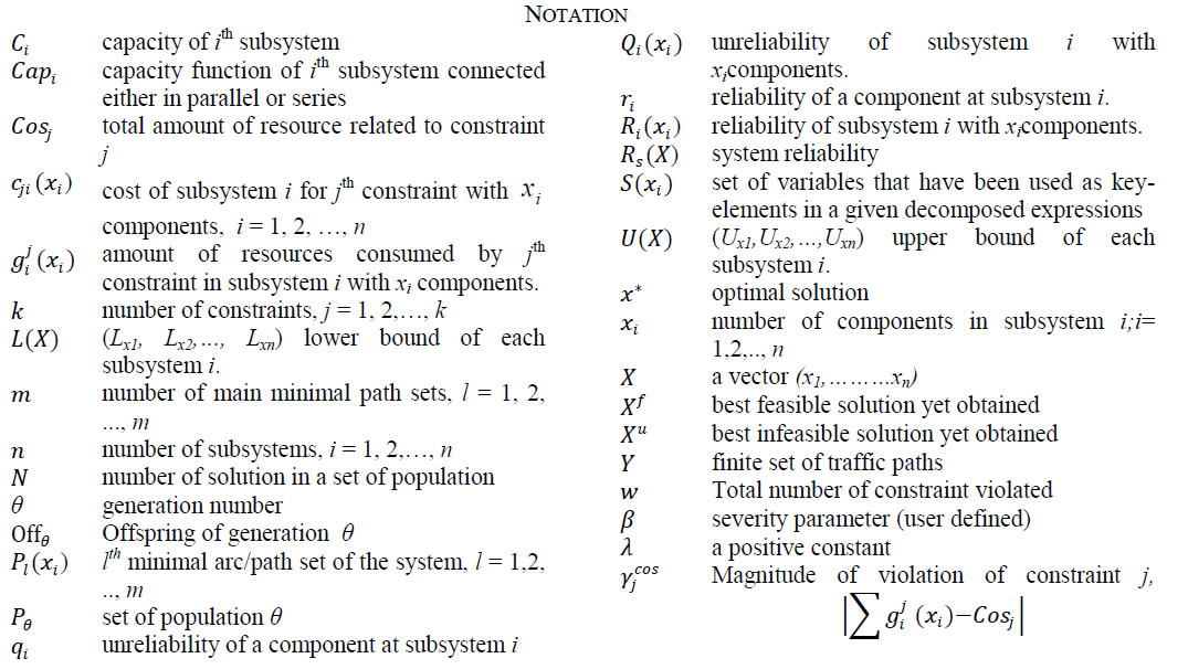 |
||||||||
ASSUMPTIONS |
||||||||
| Following are the assumptions for the rest of the sections: | ||||||||
| 1. The system and all its subsystems are coherent. | ||||||||
| 2. Subsystem structures (other than coherence) are not restricted. | ||||||||
| 3. All component states are mutually and statistically independent. | ||||||||
| 4. All constraints are separable and additive among components. | ||||||||
| 5. Each constraint is an increasing function of xi for each subsystem. | ||||||||
INTRODUCTION |
||||||||
| From the point of view of quality management and decision making, it is important to define the load carrying capacity of each node and arc of the network and develop some indexes in order to evaluate the system performance. Therefore, some researchers [1-4] have proposed models to represent such performance of flow networks and termed them as capacity related reliability (CRR) models. All these models are based on assumption that any node and arc can carry any amount of flow. However, it is not a realistic assumption. Many real life systems such as computer systems, telecommunication systems, transport systems, urban traffic systems, electrical power transmission systems, logistic supply chains, internet and flow networks etc. are mostly linked with performance. The performance of such networks, under the condition that each node and arc flow capacity is deterministic, is not only associated with network reliability but it is also the measure of maximum flow capacity per unit time between source to terminal [5].For instant, computer networks can always be modelled as flow network (FN) in which arcs/branches stands for transmission line and nodes stand for switches. All switches are assumed to be perfect i.e. any amount of flow can pass through them. Virtually each transmission line consists of several physical lines, and each physical line has several successful states hence, the capacity of each branch has several values. However, in modern flow networks or transport systems all the flow paths of a network are never active for transportation of flow from source to destination because the selection of flow paths to transport flow are decided by routing mechanism and logical links assigned in physical layer during the implementation stage. Further arcs and nodes may also be in failure or maintenance states. Hence the system capacity is not a fixed number [5]. Evaluating the probability that the system capacity is larger than or equal to the demand d (integer) with cost constraint in general is called the system reliability and is also a useful performance index to measure quality level of FN[6-11]. | ||||||||
| Many researchers [12-17] have successfully applied Genetic Algorithms (GA) to explore large, multimodal, complex problem spaces. The GA based approach can be effectively adapted for optimization of complex combinatorial problems without the knowledge of explicit mathematical treatment [13,14,16]. Hence, an advanced genetic algorithm based technique using a dynamic adaptive penalty function has been proposed. The dynamic adaptive penalty function approach considers a mix of feasible and a certain amount of infeasible solutions to guide the search from both feasible and infeasible region sides to optimal or near optimal solution of capacity related reliability of flow networks. The proposed GA to optimize CRR problems using composite performance measure (CPM) based on weighted reliability. The concept of weighted reliability was first introduced by Pahuja [18], requires that all the successful states of arcs and nodes qualifying the connectivity measure of the network be enumerated and its probability be evaluated and multiplied by the normalized weight to find out the composite performance of flow networks. The main GA steps are population reproduction, selection, crossover, and mutation. The selection, crossover, and mutation processes are repeated until the termination condition is satisfied. The proposed GA has also successfully addressed the ultrahigh reliability of modern flow networks. As only successful states are considered for computation hence higher temporal efficiency is achieved. | ||||||||
COMPOSITE PERFORMANCE MEASURE |
||||||||
| A path is a sequence of arcs and nodes connecting a source to a destination. All the arcs and nodes of network have its own attributes like delay, reliability and capacity etc.. From the quality and performance point of view, measurement of the transmission ability of a network to meet the customers demand is very important [8]. When a given amount of flow is required to be transmitted through a flow network, it is desirable tooptimize the network reliability to carry the desired flow. The capacity of each arc (the maximum flow passing the arc per unit time) has two levels, 0 and/or a positive integer value. The system reliability is the probability that the maximum flow through the network between the source and the sink is not less than the demand [6-11]. The proposed algorithm utilizes weighted reliability to form composite performance measure (CPM) to optimize the capacity related reliability (CRR) of flow networks. The weighted reliability measure [6,7,18] i.e. composite performance measure (CPM), integrating both capacity and reliability may be stated as: | ||||||||
 |
||||||||
| where | ||||||||
| is the normalized weighti.e. the ratio of capacity in the ith state to the maximum capacity of the system and Riis probability of the system being in state S(xi ) and computed as: | ||||||||
 |
||||||||
| The capacity function of different subsystems connected in parallel(Ramirez et al. 2005) [4] is: | ||||||||
 |
||||||||
| and the capacity function of different subsystems connected in series is: | ||||||||
| The rules for connecting series and parallel path sets /arcs to integrate capacity and reliability to give composite performance measure are expressed as: | ||||||||
 |
||||||||
 |
||||||||
PROBLEM FORMULATION |
||||||||
| The general constrained redundancy optimization problem in complex systems can be reduced to the following integer programmingproblem [19]: | ||||||||
| Maximize Rs(X) subject to | ||||||||
 |
||||||||
| and xi ≥ 1, for all ïÿýïÿý = 1, 2, … , n | ||||||||
| The above problem model is based on assumption that each node and arc of the network is capable of transporting any amount of flow between source and terminal. However, in present days modern flow networks the situation discussed above isnot justifiable as all the arcs are not simultaneously connected to carry flow from source to terminal. Theperformance of flow networks is considered as the reliability of maximum flow capacity and should consider immediate states of communication that manifest as performance degradation [20] by considering a simple case illustrated in Fig.1 | ||||||||
| The figure shows that there are three flow paths on the physical layer. Suppose that these flow paths, each having a capacity of 200, are used for ensuring transmission between source and terminal by load sharing. Then, the total flow capacity of the network is computed by summing the capacities of active flow paths. In this case, there are four failure modes. That is, the total capacity between two routers could be 0, 200, 400, or 600, which are recognized as being equivalent to the maximum flow in the graph. However, suppose flow paths 1 & 2 are primary flow paths with each having a capacity of 200, while flow path 3 with capacity 200 is a backup path only for flow path 1. In this case, failure modes are capacities 0, 200, or 400. These are quite different from maximum flow in graph theory.The selection of paths to transport flow is decided by routing mechanism and logical links assigned in physical layer. Thus in practical systems the entire pathsets are never utilized for transfer of information [20]. The flow is transmitted through the main path(s) only and in case of failure of main path(s), backup path(s)takes over the task of main path(s).Hence, considering the situation as discussed the general constraint reliability redundancy optimization problem expressed by equations (7) and (8) has been adapted by replacing with composite performance measure (CPM) discussed in section II (1) equations (5) and (6)above. | ||||||||
GENETIC ALGORITHM |
||||||||
| The development of GA can be termed as an adaptation of a probabilistic approach based on principles of natural evolution. Nature observes the principle of survival of fittest, weak and unfit species within their environment are faced with extinction by natural selection. The strong ones have greater opportunity to pass their genes to future generations via reproduction [21]. The genetic algorithms follow the process in which populations undergo continuous change through cross breeding, mutation and natural selection. | ||||||||
A. Steps of Genetic Algorithm: |
||||||||
| Step 1: Set θ = 1. Randomly generate N solutions to form the first population, P1. Evaluate the fitness of solutions in P1. | ||||||||
| Step 2: Crossover: Generate an offspring population Off as follows: | ||||||||
| 2.1. Randomly choose two solutions Xa∈P and Xb ∈P based on the fitness values. | ||||||||
| 2.2. Using a crossover operator, generate offspring and add them to Off | ||||||||
| Step 3: Mutation: Mutate each solution X ∈ Off with a predefined mutation rate. | ||||||||
| Step 4: Fitness assignment: Evaluate and assign a fitness value to each solution ∈ Off based on its objective function value and infeasibility. | ||||||||
| Step 5: Selection: Select N solutions from Off based on their fitness and copy them to P+ 1. | ||||||||
| Step 6: If the stopping criterion is satisfied, terminate the search and return to the current population, else, set θ = θ +1 go to Step 2. | ||||||||
| The values of its parameters, such as, population size, crossover rate, mutation rate etc. can be appropriately chosen to balance both the quality of the solution and the computational work. | ||||||||
| An initial population of a fix number of solutions is randomly selected to form the first generation of the GA. Crossover and mutation operators are then performed on the population members to produce subsequent generations. An effective GA depends on complementary crossover and mutation operators. The crossover operator dictates the rate of convergence, while the mutation operator prevents the algorithm from prematurely converging. Each member of the population is evaluated in accordance with its fitness, which is used as basis for selecting parent solutions and for culling inferior solutions from the population [14]. However, there are some difficulties in determining appropriate values for the parameters and a penalty for infeasibility. If these values are not selected properly, a GA can rapidly converge to a local optimum or slowly converge to the global optimum [13]. The population size and number of generations enhance the solution quality while increasing the computation. GA’s generally yield several good solutions (optimal or near-optimal) and thus multiple solutions obtained provide much flexibility in decision-making for reliability design. Though, these methods yield better optimal solutions at the cost of temporal efficiency. Genetic Algorithms are most suited to unconstrained optimization problems. Apart from this, sometimes for some problem GA may converge prematurely while finding optimal solution because the prior knowledge is not exploited and the local search information is not explored. Over and above this, it takes time to tune appropriately the unknown GA parameters like population size, crossover probability, maximum generation and mutation probability, to make a balance between exploitation and exploration in the search space [22]. Hence, adapting Genetic Algorithms to constrained reliability redundancy optimization problems is a challenging task. In literature, most common method in genetic algorithms to handle constraints is to use penalty functions such as Adaptive Penalties, Death Penalty, Static Penalties, Dynamic Penalties, Annealing Penalties, Segregated GA, Co-evolutionary Penalties etc. [22, 23].A new genetic search algorithm using penalty function to penalize infeasible solutions by reducing their fitness values in proportion to their degrees of constraint violation metric and its performance is presented in the following sections. | ||||||||
PENALTY FUNCTION |
||||||||
| Meta-heuristic algorithm developed is based on the approach of Bazarra et al. [24] and Yeniay [25]. The penalty function approach is used to convert the nonlinear programming problem with equality and inequality constraints into an unconstrained problem, or into a problem with simple constraints [26]. This is achieved by including the constraints into the objective function via a penalty parameter to penalize any violation of the boundaries/constraints. It is generally difficult to find an effective and efficient penalty function, which can inherit the constraints. Defining penalty function for solving a problem varies with the type of the problem. | ||||||||
| The combination of distance metric together with the length of the search has been very effective for this type of search problems. The algorithm developed is based on an adaptive penalty function and the search pattern Agarwal and Gupta [16, 26]. During iterations the penalty function adapts itself according to the deviations of current solution from the best feasible/infeasible solution obtained by the algorithm. This helps the search not to go too far into the infeasible region. It also incorporates the ratio of the count of constraints violated to the total number of constraints as one of the distance metric. The algorithm also incorporates the number of iterations elapsed as length of search in penalty function; hence justifying the name dynamic adaptive penalty function. Although GA algorithms have proven to be efficient for solving reliability redundancy optimization of system, one of their major disadvantages is the increase of computational effort involved. | ||||||||
| The general penalty function approach is as follows. | ||||||||
 |
||||||||
| where A and B are limits of search space. The problem can be reformulated as state: | ||||||||
| Subject to x∈ A | ||||||||
| where is a function measuring the distance of the vector X from the region B, p is a monotonically nondecreasing penalty function such that p(0) = 0. Measure of various distance metrics (d) include a count of violated constraints, the Euclidean distance between X &B, a linear sum of the individual constraint violations, or this sum raised to some exponent β a user defined severity parameter [16, 26, 27]. | ||||||||
| On the basis of above discussions, the dynamic adaptive penalty function is designed to solve the constrained reliability redundancy optimization problems of complex systems. It is an adaptation of penalty function used by [16] for series parallel systems to complex systems. It accounts for the amount of infeasibility and the maximum improvement possible in the current solution of a generation, and exhibiting severity of the penalty imposed. | ||||||||
 |
||||||||
The adapted/penalized composite performance measure is a function of composite performance measure CPM and the severity of the constraints. The metric (w/k ) calculates the ratio of the number of constraints violated to the total number of constraints. The distance metric evaluates the sum of the ratios of magnitudes of constraint violations to total resources available incorporating the dynamic aspect, and increases the severity of the of constraint violations to total resources available incorporating the dynamic aspect, and increases the severity of the (taken as 0.005 after experimentation), and θ the generation number. The adaptive term evaluates the sum of the ratios of magnitudes of constraint violations to total resources available incorporating the dynamic aspect, and increases the severity of the of constraint violations to total resources available incorporating the dynamic aspect, and increases the severity of the (taken as 0.005 after experimentation), and θ the generation number. The adaptive term  takes care of the maximum possible improvement in the current solution with respect to the difference between the un-penalized values of the best infeasible and feasible solutions obtained up to the time, takes care of the maximum possible improvement in the current solution with respect to the difference between the un-penalized values of the best infeasible and feasible solutions obtained up to the time, |
||||||||
| When |
||||||||
BOUNDS FOR SYSTEM |
||||||||
| The bounds to each of the subsystem determine the region of search. The lower bound to the system is generally known from the system design. For systems with heterogeneous redundancy allocation lower bound vector is taken as: L = (1, 1, …, 1) for all xi . While the upper bound is determined from the constraints, allocating the whole resource of constraint j to xi, and determine the maximum value of xi while keeping all other subsystems at their lower bounds. | ||||||||
STOPPING FUNCTION |
||||||||
| In this algorithm two stopping criteria, i.e., number of generations and/or the desired system reliability are considered. The number of generation is considered as one of the stopping criteria for the algorithm and this is user or problem dependent. The second criterion for terminating the algorithm is the desired value of the system reliability. | ||||||||
COMPUTATION AND RESULTS |
||||||||
| To illustrate the performance of the proposed algorithm a network having six arcs {x1, x2, x3, x4, x5, x6} and five minimal path sets {y1, y2, y3, y4, y5} as shown in the Figure.2 is considered and solved for capacity related constraint redundancy reliability optimization using CPM. The network shown in Fig. 2 is a bench mark problem, considered by Hayashi & Abe (2008) [20]. | ||||||||
| Using Baye’s method, the Reliability of the system can be expressed as: | ||||||||
 |
||||||||
| The problem is solved for data given in Table 1 and by assuming that each flow path has a capacity of 100. The total flow through network at any time should not be less than 200 in any case. | ||||||||
| The procedure to implement the search using genetic algorithm is as follow: | ||||||||
A. Chromosome representation: |
||||||||
| Chromosome representation is a crucial part of any genetic algorithm. There are several ways of chromosome representation for any given problem. The GA works with the binary encodings, but for many industrial problems binary string is not a natural coding. Hence various non-string techniques have been used for such problems: real number coding for constrained optimization problems and integer coding for combinatorial problems. For the nonlinear integer programming problems of the type given by (1), the integer encoding as a vector representation is more efficient. | ||||||||
B. Generation of initial population: |
||||||||
| A fixed number of chromosomes are randomly generated to form an initial population. In a chromosome, a gene at any locus is randomly generated integer between the lower limit and upper limit defined for each subsystem. Population size of 100 is taken for each of the test problems. | ||||||||
C. Evaluating the fitness of chromosomes: |
||||||||
| The fitness of the chromosomes is found by using penalized objective function value using (5). | ||||||||
D. Genetic Operators: |
||||||||
| Two genetic operators Crossover and Mutation are the backbone of any GA. Using these two operators new off springs of the genes are created at each generation. | ||||||||
1) Crossover Operator: |
||||||||
| It provides a thorough search of regions of the sample space to produce good solutions. For this GA, crossover rate pc, denoting the expected number of chromosomes that undergo crossover, is taken as 0.5 for the system structures. However, depending on the size of the system, it can be varied. The total population is arranged in decreasing order of fitness i.e. fittest to the least fit chromosome. A random number p is generated such that 0 ≤ p ≤ 1 for each of the population member and a chromosome is selected as a parent if and only if p < pc. If the number of such selected chromosomes is odd then the last chromosome selected as parent is dropped from the mating pool. Single-point crossover method is used to mate the parents and cut position is generated randomly from the interval [1, n]. | ||||||||
2) Mutation: |
||||||||
| Mutation operator produces random changes in various chromosomes. The mutation rate is the rate pm controls the rate at which new genes are introduced into the population for trial. If it is too low, then some genes that would have been useful are never tried out, but if it is too high, then there will be much random perturbation and the off springs will start losing their resemblance to the parents and the algorithm will lose the ability to learn from history. For the present GA, pm is taken as 0.20. Random number p is generated for each gene within the interval from interval [0, 1] as 0 ≤ p ≤ 1. If p < pm then the gene is randomly flipped to another gene from the corresponding set of alternatives (To reach upon the effective values of the parameters pc and pm brief experiments were conducted). | ||||||||
E. Selection: |
||||||||
| Each generation after undergoing genetic operations produces good or bad solutions. All the solutions (initial population, children and off springs) are arranged in descending order of fitness and the population is selected for the next generation. | ||||||||
| The algorithm has been programmed using MATLAB and tested on a Core i7 VPro 3.4 GHz system. Execution time for the problem is determined. The proposed genetic algorithm gives the optimal solution (2, 2, 2, 2, 1, 3) with system reliability Rs = 0.9578, the optimized subsystem reliability probability Ri and unreliability probabilities Qi are shown in Table 2. | ||||||||
| The capacity of each subsystem of the flow path is taken as 100 and the capacity of flow paths of the network is determined using (3) of proposed approach. The optimized arc capacity and value of composite performance measure CPM are illustrated in Table 3.Thevalue for CPM for an assumed flow of 200 is supposed to pass through the flow path and it comes out to be 1.0000 as shown below: | ||||||||
 |
||||||||
| To demonstrate the adaptability of the penalty function to constrained redundancy optimization of flow networks problem with respect to β, the different values β (1.0 ≤ β ≤ 8.0) are used to determine the best feasible solution, average reliability, standard deviation and average time consumed in 10 GA trials. The best value of β for a particular problem is the value of β giving the best feasible solution, highest average reliability, least standard deviation and least average time. These values are shown in the Table 4. | ||||||||
| The values of β (1.0, 2.0 or 3.0) give the same best feasible solution (2 2 2 2 1 3) with system reliability Rs= 0.9578 and zero standard deviation parameter. However, the same solution and system reliability values in all the 80 GA trials with least average time is obtained for β = 8, but the standard deviation in this case is more in comparison to the cases for β = 1.0, 2.0 or 3.0. The average time consumed is comparable and average reliabilities are same for the selected values of β. It can be noted that higher values of β increases the standard deviation.The above result shows that proposed method is capable of optimizing the flow network to transport the desired capacity through the network with best feasible solution, highest average reliability, best average time and least standard deviation. | ||||||||
CONCLUSIONS |
||||||||
| The GA method developed in this study give very promising results. The algorithm attack the search for optimal solution from both infeasible and feasible region sides which is a superior strategy to keep the solution in feasible region for constrained redundancy reliability optimization of flow networks. For the search to precede efficiently toward the final optimal /near optimal solution a dynamic adaptive penalty function using distance based metric, has been utilized. The demonstrations show that GA approach can be a powerful tool for solving problems of constrained redundancy optimization of flow networks. The numerical example demonstrates that the proposed algorithm is fast for designing large, reliable telecommunications networks. | ||||||||
Tables at a glance |
||||||||
|
||||||||
Figures at a glance |
||||||||
|
||||||||
References |
||||||||
|

