ISSN ONLINE(2278-8875) PRINT (2320-3765)
ISSN ONLINE(2278-8875) PRINT (2320-3765)
| M. Anuj Gargeya and Sai Praneeth Pabba Department of Electrical and Electronics Engineering, GITAM University, Hyderabad, India |
| Related article at Pubmed, Scholar Google |
Visit for more related articles at International Journal of Advanced Research in Electrical, Electronics and Instrumentation Engineering
In a practical power system, the power plants are not located at the same distance from the centre of loads and their fuel costs are different. Also, under normal operating conditions, the generation capacity is more than the total load demand and losses. Thus, there are many options for scheduling generation. In an interconnected power system, the objective is to find the real and reactive power scheduling of each power plant in such a way as to minimize the operating cost. This means that the generator‟s real and reactive powers are allowed to vary within certain limits so as to meet a particular load demand with minimum fuel cost. This is called optimal power flow problem. In this project, ECONOMIC LOAD DISPATCH (ELD) of real power generation is considered. Economic Load Dispatch (ELD) is the scheduling of generators to minimize total operating cost of generator units subjected to equality constraint of power balance within the minimum and maximum operating limits of the generating units. In general by neglecting valve point loading effects, economic load dispatch can be solved either by lambda search or generation search (Pg) methods. In this project, valve point loading effects of the generating units are considered. To solve economic load dispatch, two of intelligent search methods are considered, namely, genetic algorithm and pattern search methods. Equality constraint is satisfied by penalty approach method.Economic load dispatch solved for three typical test cases of 5 generator, 13-generator and 40-generator (Tai-power systems) cases.
Keywords |
| Economic Load Dispatch, Fuel cost function, Genetic Algorithm, Pattern search method, Tai-power systems. |
INTRODUCTION |
| The efficient and optimum economic operation and planning of electric power generation systems have always occupied an important position in the electric power industry . Prior to 1973 and the oil embargo that signalled the rapid escalation in fuel prices, electric utilizes in the united states spent about 20% of their total revenues on fuel for the production of electrical energy. By 1980 that figure has risen, to more than 0% of the total revenues. In the 5years after 1973, US electric utility fuel costs, escalated at a rate that averaged 25% compounded on the annual basis, the efficient use of available fuel is growing in importance, both monetarily and because most of the fuel used represents irreplaceable natural resources. An idea of magnitude of the amounts of money was under consideration, can be obtained by considering the annual operating expenses of a large utility for purchasing fuel. Assume the following parameters for the moderately large system. |
| Annual peak load= 10,000mw |
| Annual load factor= 60% |
| Average annual heat rate for converting fuel to electric energy= 10,000Btu/kwh |
| Average fuel cost= $3.00/million Btu, corresponding to oil priced at 18$/Bbl |
| With these assumptions, the total annual fuel cost for the system is as follows |
| Annual energy produced =10^7 mw * 8760hr/year * 0.60 = 5.256 * 10^10kwh |
| Annual fuel consumption= 10,500 Btu/kwh * 5.356 * 10^10 kWh = 55.188 * 10^13 Btu |
| Annual fuel cost = 55.188* 10^13 * 3* 10^-6 $/Btu = $1.66billion |
| To put this cost in perspective, it represents a direct requirement for revenues for the average customer of the system of 3.15cents/kwh just to recover the expense for fuel. A savings in the operation of the system of small percent represents a significant reduction in operating cost, as well as in the quantities of fuel consumed. It is no wonder that this area has warranted a great deal of attention from the engineers through the years. |
| Periodic changes in basic fuel price levels serve to accentuate the problem and increase its economic significance. Inflation also causes problems in developing and presenting methods, techniques, and examples of economic operation of electric power generating systems. Recent fuel cost always seem to be ancient history and entirely in an appropriate to current conditions. |
INTRODUCTION OF INTELLIGENCE TECHNIQUES |
| Rapid growth in power system size and Electrical power demand, problem of reducing the operating cost has gained importance while maintaining voltage security and thermal limits of transmission line branches. A large number of mathematical programming and Artificial Intelligence Technique have been applied to solve (Economic Load Dispatch) ELD. In most general formulation, the ELD is a nonlinear, non-convex, large scale, static optimization problem with both continuous and discrete control variables. Mathematical programming approaches most general formulation, the ELD is a nonlinear, non-convex, large scale, static optimization problem with both continuous and discrete control variables. |
FUEL COST FUNCTION |
| The components of the cost that fall under the category of dispatching procedures are the costs of the fuel burnt in the fossil plant because nuclear plants tend to be operated at constant output levels and hydro plants have essentially no variable operating costs. The total cost of operation includes the fuel cost, costs of labour, supplies and maintenance. Generally, costs of labour, supplies and maintenance are fixed percentages of incoming fuel costs. We assume that the variation of fuel cost of each generator (Fi) with the active power output (Pi) is given by a quadratic polynomial. |
 |
| Where, |
| Fi = fuel cost of generator i. |
| Pi = power output of generator i |
| ai = measure of losses in the system. |
| bi = represents the fuel cost. |
| ci = includes salary and wages, interests and depreciation |
| And is independent of generation |
| NG = number of generation buses |
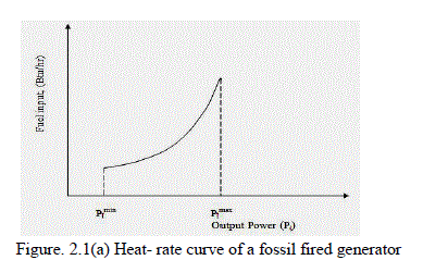
| Input of thermal plant is generally measured in Btu/hr and the output is measured in MW. A simplified input output curve of the thermal unit known as heat rate curve is given in following fig.2.1 (a). |
 |
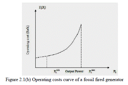
| Converting the ordinate of heat rate curve from Btu/hr to Rs/hr, results in the operating cost curve shown in fig. 2.1(b). |
 |
INCREMENTAL FUEL COST |
| In economic evaluation, there is a great tendency to resort to average rates to arrive at a total cost. Extreme caution should be exercised in doing this, especially in dealing with unit fuel cost of energy produced by a generating station. The additional fuel cost of energy produced depends entirely upon the manner in which the generation is added. The input and output curve of generating units of thermal plants is shown in fig 2.2, The abscissa is output power Pi in MW, x-ordinate as fuel (heat) input in joules per hours of the ith unit. The ordinate of curve may be converted to fuel cost in Fi Rs/hr by multiplying the fuel input by the fuel is Rs/joule. |
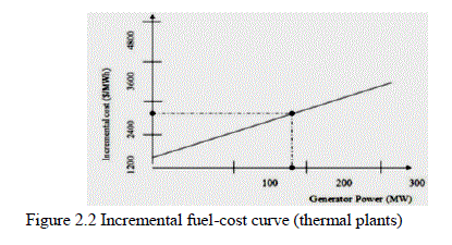 |
| The slope of cost curve at a point M is given by |
 |
| Where, ΔFi = increase in fuel cost corresponding to an increase of power output ΔPi. The increment fuel cost for a generator for any given electrical power output is defined as the limiting value of the ratio of the increase in cost of fuel in Rs/h to the corresponding increase in electrical power output tends to zero. |
MATHEMATICAL FORMULATION |
| The ELD problem is defined as to minimize the total operating cost of a power system while meeting the total load plus transmission losses within generator limits. Mathematically the problem is defined as (including losses) |
| Minimize: |
 |
| Subject to (1) the energy balance equation |
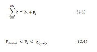 |
| Where, |
| ai, bi, ci : cost coefficients |
| PD: load demand |
| Pi: real power generation |
| PL: power transmission |
| NG: number of generation busses |
GENETIC ALGORITHM |
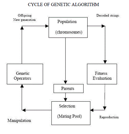
| INTRODUCTION: Genetic Algorithms (GAâÃâ¬ÃŸs) are based on analogy , and are adaptive heuristic search algorithm based on , evolutionary ideas of natural selection and genetics. As such , they GAâÃâ¬ÃŸs represent an intelligent exploitation of the random search used , to solve search and optimization problems. Although randomized, GAâÃâ¬ÃŸs are by no means random, instead they are exploit historical information to direct the search in to the region of better performance with in the search space. The basic techniques of the GA are designed to simulate processes in natural systems necessary for evolution, especially those follow the principles first laid down by Charles Darwin of , "Survival Of The Fittest". Since in nature, competition among individuals for scanty resources , results in the fittest individuals dominating over the weaker ones. |
| Genetic Algorithms are better than conventional algorithms in that they are more robust. They do not break easily , even if the inputs are changed slightly , or in the presence of reasonable noise. Also, in searching a large state-space, multi-modal state-space, or n-dimensional surface, a genetic algorithm may offer significant benefits over more typical search of optimization techniques such as linear programming, heuristic, depth-first, breathfirst, and praxis. |
| GAâÃâ¬ÃŸs are based on an analogy , with the genetic structure and behavior of chromosomes with in a population of individuals using the following foundations: |
| • Those individuals most successful in each 'competition' will produce more offspring than those individuals that perform poorly. |
| • Genes from „goodâÃâ¬ÃŸ individuals propagate throughout the population , so that two good parents will sometimes produce offspring that are better than either parent. |
| • Thus , each successive generation will become more suited to their environment. |
 |
| GENERAL GENETIC ALGORITHM: |
| The general GA is as follows: |
| STEP1: CREATE A RANDOM INITIAL STATE: An initial population is created from a random selection of solutions .this is unlike the situation for symbolic AIsystem, where the initial state in a problem isalready given. |
| STEP2: EVALUATE FITNESS: A value for fitness is assigned to each solution depending on how close it actually is solving the problem. These solutions are not to be confused with answers of the problem; think of them as possible characteristics that the system would imply in order to reach the answer . |
| STEP3: REPRODUE (AND CHILDREN MUTATE): Those chromosomes with a higher fitness value are more likely to reproduce offspring .The offspring is a product of the father and mother, whose composition consists of a combination of genes from the two This process is known as crossing over . |
| STEP 4: NEXT GENERATION :If the new generation contains solution that produces an output that is a close enough or equal to the desired answer then the problem has been solved . if this is not the case ,then the new generation will go through the same process as their parents did. This will continue until a solution is reached. |
PATTERN SEARCH |
| Pattern search (PS) is a family of numerical optimization methods that do not require the gradient of the problem to be optimized. Hence PS can be used on functions that are not continuous or differentiable. Such optimization methods are also known as direct-search, derivative-free, or black-box methods. |
| They varied one theoretical parameter at a time by steps of the same magnitude, and when no such increase or decrease in any one parameter further improved the fit to the experimental data, they halved the step size and repeated the process until the steps were deemed sufficiently small. |
| PERFORMING A PATTERN SEARCH: |
| CALLING PATTERN SEARCH AT THE COMMAND LINE: |
| To perform a pattern search on an unconstrained problem at the command line, call the function pattern search with the syntax [x fval] = pattern search (@objfun, x0) |
| Where, |
| • objfun is a handle to the objective function. |
| • x0 is the starting point for the pattern search. |
| The results are: |
| • x - Point at which the final value is attained. |
| • fval - Final value of the objective function. |
| PLOTTING THE OBJECTIVE FUNCTION VALUES AND MESH SIZES: |
| To see the performance of the pattern search, display plots of the best function value and mesh size at each iteration. First, select the following check boxes in the Plots pane: |
| • Best functionvalue |
| • Mesh size |
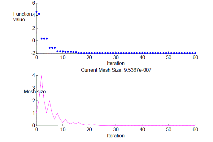 |
| The upper plot shows the objective function value of the best point at each iteration. Typically, the objective function values improve rapidly at the early iterations and then level off as they approach the optimal value. |
| The lower plot shows the mesh size at each iteration. The mesh size increases after each successful iteration and decreases after each unsuccessful one. |
RESULTS |
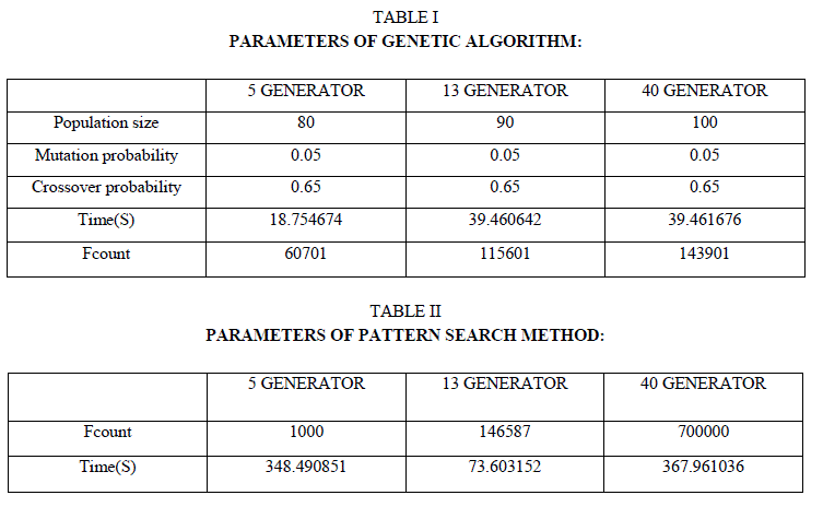
| Proper choice of genetic algorithm parameters is the first task in deciding the test performance of genetic algorithm. Parameters include population size, crossover, mutation probabilities and type of best fitness value selection. In each case numbers of trails are made to arrive at these parameters. |
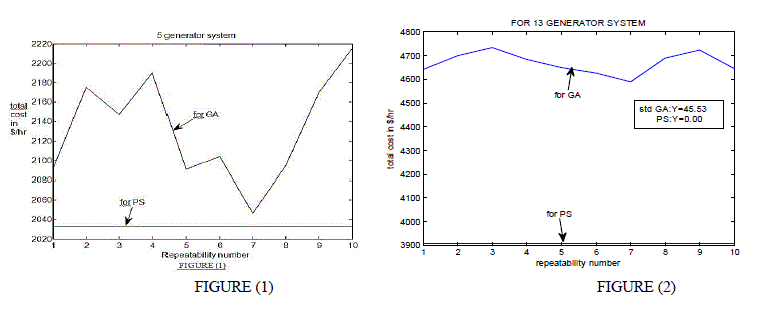
| In case of 5generator case population are varied in multiple proportions of number variables of the optimization problem. Final population size is indicated in table (1) after increasing and decreasing population size from the value indicated. For all the cases considered fitness value selection is done by a property of elitism. Mutation and crossover probabilities are set to 0.05 and 0.65 respectively. In table (1) number of function counts made for each test case is indicated. ItâÃâ¬ÃŸs clear from table (1) that as number of design variables increases the function count increases to search the optimum value to the specified tolerance of constraint. Time of computation also increases as the design variables increases. On contrary to the genetic algorithm, pattern search does not require any parameters. Pattern search performs, local search by reduction in size of the search space in Pg number of univariate directions and hence possibility of number of function evaluations increases. This function count and time of computing the search is indicated in table (2). Any simulation, particularly a stochastic and random method should arrive at same results upon repetition of simulations. To test the reliability, for genetic algorithm and pattern search is run 10 times for same load condition (5 generator-650MW, 13 generators -1100MW, 40 generators- 7500MW). |
 |
| REPEATABILITY FOR 5 GENERATOR SYSTEMS (Figure 1) |
| REPEATABILITY FOR 13 GENERATOR SYSTEMS (Figure 2) |
| REPEATABILITY FOR 40 GENERATOR SYSTEMS (Figure 3) |
 |
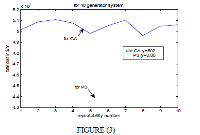 |
| The result of such simulation is shown in fig (1), fig (2) and fig (3) respectively. From curve drawn indicates on x axis major repetition number on y axis, the final total cost ($/hr).The data statistics of curve such as standard deviation is a measure of variation of the optimization method. It is clear from the graphs of repeatability simulation that pattern search is highly reliable compare to genetic algorithm. |
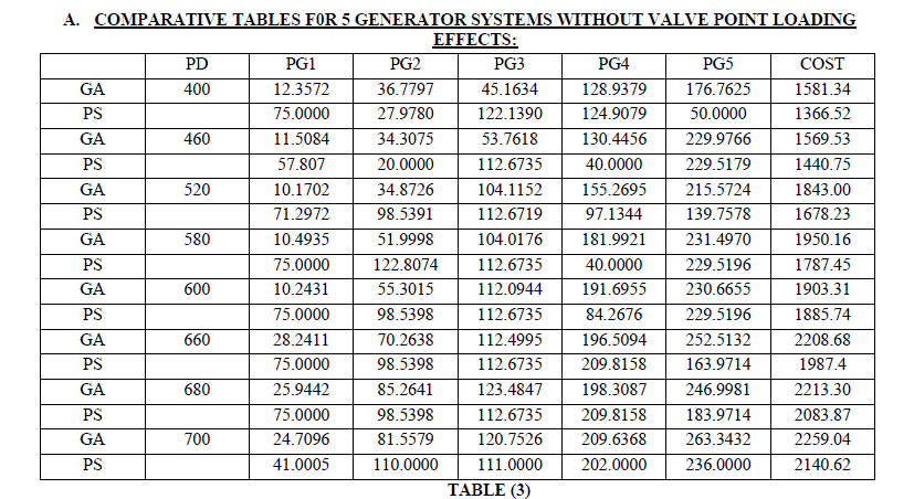
| After simulations are carried out for the three test cases by varying real power demand using both methods i.e., Both optimization methods from graphs shown in fig(4),fig(5) indicates the effects of valve points is to increase the cost of power production way. The below are the results obtained for 5 generator systems by using both GA and PS method: |
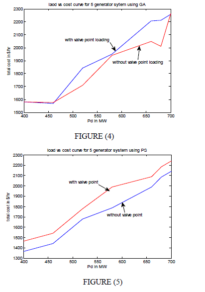 |
| FOR 5 GENERATOR SYSTEMS (Figure 4) by using GA Method |
| FOR 5 GENERATOR SYSTEMS (Figure 5) by using PS Method |
 |
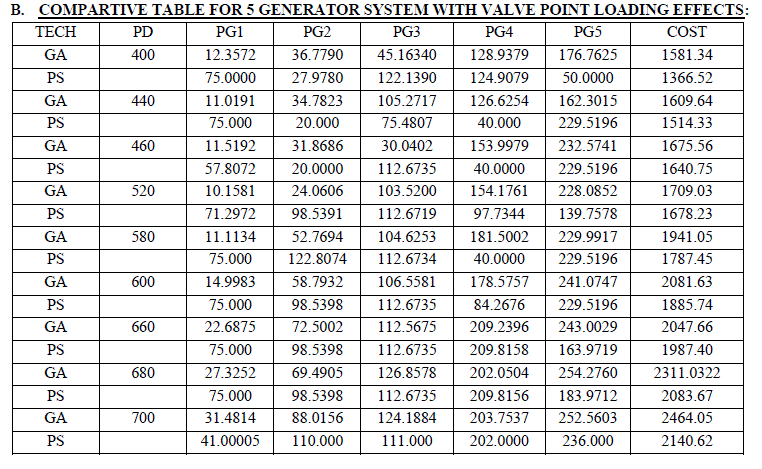 |
| • Pd and Pg’s are in MW |
| • COST is in $/hr |
CONCLUSION |
| Economic load dispatch is solved by using GENETIC ALGORITHM and PATTERN SEARCH method without considering losses. Both GA and PS are applied for a practical test system of 5 generator, 13 generators and TAI power system with and without valve point loading effects. With valve point loading effects the cost function of generator consists of valley points which offer a challenge for optimization method to search for better solutions without being struck at break (valley) points. Both optimization methods of this project work have following conclusions to offer. |
| • With valve point effects, cost of generation increases. |
| • PATTERN SEARCH being invariable search indifferent meshes of function contour resulted in best cost but at the cost of more function evaluations than GENETIC ALGORITHM. |
| • Constraint satisfaction i.e. variable penalty function method is found to be effective both in GA and PS .In both these cases constraint satisfaction is considered as 1*10^-5. |
| • Upon observation of time of computation it is suggested to develop a regression model or Artificial Neural Network (ANN) for instants solutions. To obtain training data for regression or ANN training instances can be obtained from PS. |
References |
|