Energy Forecasting using Artificial Neural
Networks

G.Tamizharasi; S.Kathiresan; K.S.Sreenivasan

Energy Forecasting using Artificial Neural Networks

G.Tamizharasi¹, S.Kathiresan² and K.S.Sreenivasan³

Assistant Professor, Dept. of E&I,Bharath University,Chennai-600073, India
Professor,Departmentment of Mechanical Engineering,Karpaga Vinayaga College of Engg and Tech, Chennai
Asst. Professor, Department of Mechanical Engineering, Karpaga Vinayaga College of Engineering and Technology, Chennai

Related article at Pubmed, Scholar Google

Visit for more related articles at International Journal of Advanced Research in Electrical, Electronics and Instrumentation Engineering

Abstract

Artificial Neural Network (ANN) has been used in nonlinear systems modeling and simulation. One of the most useful and interesting factors of ANNs is forecasting. This paper discusses the application of ANNs to predict the long range energy consumption for a country. In this study the long-term energy consumption for the years ahead is predicted, exploiting ANN computational speed, ability to handle complex non-linear functions, robustness and great efficiency even in cases where full information for the studied problem is absent.

Keywords

Artificial Neural Network, Energy Forecasting

INTRODUCTION

In recent years, much research has been conducted on the application of artificial intelligence techniques to forecast short term consumption, such as hourly or daily load forecasting and medium term forecasting because of the ANN’s ability to learn and construct a complex nonlinear mapping through a set of input/output examples. However, the general style of long term energy consumption forecasting has emphasized aggregate energy consumption forecasting up to now, and consequently, regression based and time series models have been used because of the smoothing of time in the accumulation process. Recently, ANNs have been used in regression based and time series models. They have been used in the areas of electricity price forecasting, load forecasting and power factor correction techniques. ANNs can be used for long term forecasting, such as annual forecasting, in spite of its heterogeneity and strong and nonlinear changes of demand in high energy consumption industries, which makes forecasting a cumbersome and vague task. Therefore, the nonlinear structure of energy intensive industries makes the ANN an ideal candidate for forecasting estimations.

The multilayer perceptron model (MLP) has been used for this purpose. Several possible architectures are tested and the one with the best generalizing ability. Actual recorded input and output data that influence long-term energy consumption were used in the training, validation and testing process. The developed ANN model is used for the prediction of 2005–2008, 2010, 2012 and 2015 energy consumption producing very accurate results comparing them with the results of a linear regression method, a support vector machine method and the actual available recorded data for years 2005–2008. The proposed approach can be very useful in the effective implementation of energy policies. Furthermore the proposed approach could be an accurate tool for the long-term energy consumption prediction problem.

An artificial neural network consists of a number of very simple and highly interconnected processors, called neurons, which are analogous to the biological neurons in the brain. The neurons are connected by weighted links that pass signals from one neuron to another. Each link has a numerical weight associated with it. Weights are the basic means of long-term memory in ANN. They express the strength, or importance, of each neuron input. A neural network ‘‘learns’’ through repeated adjustments of these weights. The characteristic feature of these networks are that they consider the accumulated knowledge acquired during training and respond to new events in the most appropriate manner, giving the experience gained during the training process. In this work a typical neural network model known as multilayer perceptron model (MLP) has been used.

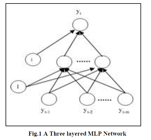
The MLP is a feed forward neural network with an input layer of source neurons, at least one middle or hidden layer of computational neurons, and an output layer of computational neurons (Fig. 1). The input layer accepts input signals from the outside world and redistributes these signals to all neurons in the hidden layer. The hidden layer detects the feature. The weights of the neurons in the hidden layers represent the features in the input patterns. The output layer establishes the output pattern of the entire network. In order to train the network, a suitable number of representative examples of the relevant phenomenon must be selected so that the network can learn the fundamental characteristics of the problem. More than a hundred different learning algorithms are available, but the most popular one is the back propagation. In a back propagation neural network the learning algorithm has two phases. First a training input data set is presented to the network input layer. The network then propagates the input data set from layer to layer until the output data set is generated by the output layer. If this data set is different from the desired output, an error is calculated and then propagated backwards through the network from the output layer to the input layer. The weights are modified as the error is propagated.

ANN MODELS

ANN models are determined according to their architecture, i.e., the network’s structure, transfer function and learning algorithm. In the back propagation networks the MLP architecture is generally decided by trying a) varied combinations of number of hidden layers and number of nodes in a hidden layer, b) different transfer functions and c) learning algorithms in order to be selected the most suitable ANN model architecture, which has the best generalizing ability amongst the all tried combinations, i.e., minimization of the sum-squared error. Once the training process is completed and the weights and bias of each neuron in the neural network is set, the next step is to check the results of training by seeing how the network performs in situations encountered in training and in others not previously encountered.

Although there are several different types of artificial neural networks in this study the back propagation MLP model has been used. The main reasons were: a) small solution network and quick computational speed that permits training over large input data sets, b) automatic generalization of knowledge enabling the recognition of data sets, c) robustness to recognize data obscured by noise, d) minimization of the mean squared aggregate error across all training data sets and e) supervised training. The main disadvantage of the back propagation MLP is the many variables which must be considered when constructing a MLP. This includes the number of hidden layers, the type of transfer function(s), the initial conditions, and the types of back propagation MLPs available. One must also consider the training time which is a direct function of training set size and MLP chosen for the task.

The input nodes are the previous lagged observations, while the output provides the forecast of the future value. Hidden nodes with appropriate nonlinear transfer functions are used to process the information received by the input nodes. The model can be written as:

where m is the number of input nodes, n is the number of hidden nodes, f is a sigmoid transfer function, such as the logistic function: f(x) = 1/(1+exp (-x)) . { αj, j = 0,1,. . . , n} is a vector of weights from the hidden to the output nodes and {βij, i = 1, 2, . . ., m; j = 0, 1, . . ., n} are weights from the input to the hidden nodes. α0 and βoj are the weights of arcs leading from the bias terms, which have values always equal to 1. Note that Eq. (1) indicates a linear transfer function employed for the output node as desired for forecasting problems. The MLP’s most popular learning rule is the error back propagation algorithm. At the beginning of the learning stage, all weights in the network are initialized to small random values.

The algorithm uses a learning set, which consists of input– desired output pattern pairs. Each input–output pair is obtained by off line processing of historical data. These pairs are used to adjust the weights in the network to minimize the sum squared error (SSE), which measures the difference between the real and the desired values overall output neurons and all learning patterns. After computing SSE, the back propagation step computes the corrections to be applied to the weights. ANN models have been researched in connection with many power system applications, short term forecasting being one of the most typical areas. Most of the suggested models use MLP networks. The attraction of MLP networks has been explained by the ability of the network to learn complex relationships between input and output patterns, which would be difficult to model with conventional algorithmic methods.

ANN SOLUTION

There are three steps in solving an ANN problem, (1) training, (2) generalization and (3) implementation. Training is a process by which the network learns to recognize the present pattern from the input data set. We present the network with training examples, which consist of a pattern of activities for the input units together with the desired pattern of activities for the output units. For this reason, each ANN uses a set of training rules that define its training method. Generalization or testing evaluates the network’s ability to extract a feasible solution when the inputs are previously unknown to the network and have not been used to train the network. We determine how closely the actual output of the network matches the desired output in new situations. In the learning process, the values of the inter-connection weights are adjusted so that the network produces a better approximation of the desired output. ANNs learn by example. They cannot be programmed to perform a specific task. The examples must be selected carefully, otherwise useful time is wasted or, even worse, the network might be functioning incorrectly. The disadvantage is that because the network finds how to solve the problem by itself, its operation can be unpredictable. In this case, the effort is made to identify the best suited network for the desired model according to the characteristics of the problem and the ANN features.

ENERGY CONSUMPTION

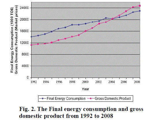
Energy forms a key part of human’s everyday lives. Energy is needed in almost every activity. As economy grows, demand for energy dramatically increases. According to the American Energy Information Administration (AEIA) and to the International Energy Agency (IEA), the world-wide energy consumption will on average continue to increase by 2.5% per year and this forms a modest prediction. In this case, the final energy consumption which includes all energy delivered to the final consumer’s door (industry, transport, households and other sectors) for all energy uses, has increased the last 16 years more than 60%, from 14,079,000 Tones of Oil Equivalent (TOE) in 1992 to 22,552,000 TOE in 2007 following an average annual increase of approximately 4.1%. Fig. 2 presents the final energy consumption in comparison to the gross domestic product (GDP) of a country from 1992 to 2007, showing clearly the relation of economy and energy consumption.

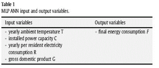Fig. 3 indicates installed power capacity in MW and the yearly per resident electricity consumption in kWh have increased significantly the last 16 years .Their continuous increase which is not expected to be stabilized or to be decreased would certainly have a great influence on the long-term energy consumption. A very crucial factor that also affects energy consumption is climate. The yearly ambient temperature increase has a considerable effect in the energy consumption for very obvious reasons, i.e., increase in temperature leads to a higher use of air-conditioners and other cooling devices. Recent studies have concluded that the sensitivity of energy consumption to temperature has increased in the recent period. Given the concern about global warming, these findings support the renewed interest in energy related questions by the policymakers.

DESIGN OF THE PROPOSED MLP ANN MODEL

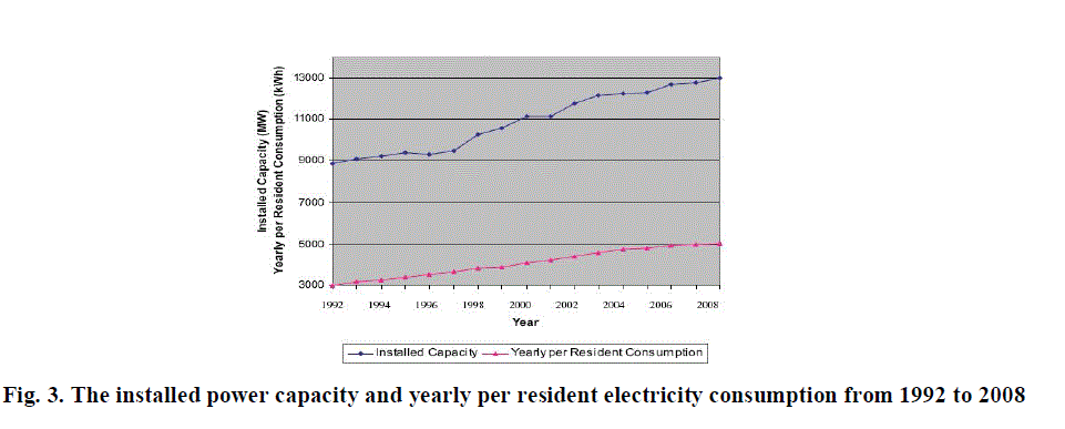
The goal of this study is to discuss about an artificial neural network architecture capable to predict the long-term energy consumption. The four parameters analyzed in the previous section, that play important role to the long-term energy consumption were selected as the inputs to the neural network, while as output the final energy consumption was considered.

These parameters, summarized in Table 1, constitute actual recorded data. More specifically, the yearly ambient temperature T has been supplied from the Meteorological Service, the installed power capacity C and the yearly per resident electricity consumption R have been supplied from Public Power Corporation, while the gross domestic product G has been supplied from EUROSTAT. Finally the output variable, i.e., the final energy consumption F has been also provided from EUROSTAT. It must be mentioned that the author has selected only those four input parameters for the designed ANN model, although there are also others (e.g. amount of CO2 pollution, number of air conditioners, installation of renewable energy technologies, electricity price, etc.), that affect the energy consumption. As it has stated earlier each ANN model is determined according to its structure, the transfer function and the learning algorithm, which are used in an effort to learn the network the fundamental characteristics of the examined problem. In this case, thousands of MLP ANN models were designed and tested. These were combinations of five back propagation learning algorithms, five transfer functions and structures consisted of 1 to 5 hidden layers with 2 to 100 neurons in each hidden layer (Table 2).

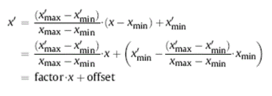
The MATLAB_ neural network toolbox was used to train the developed neural network models. Input and output data of the last 13 years (1992–2004), were used to train and validate the neural network models. In each training iteration 20% of random samples were removed from the training set and validation error was calculated for these data. The training process was repeated until a root mean square error between the actual output and the desired output reached the goal of 1% or a maximum number of epochs (the presentation of the set of training data to the network and the calculation of new weights and biases) it was set to 15,000, was accomplished. Finally, the predicted energy consumption value was checked with values obtained from situations encountered in the training and others which have not been encountered. It must be mentioned that prior the ANN training, data normalization was performed. This was necessary not only because all entries need to be guaranteed to have the same weight, but also because the range of values must be limited for neuron’s transfer function in order the network to converge in training and produce meaningful results. Although several normalization methods exist, common feature of all these is that an offset is deducted from the data items, after which they are transformed over the desired range by means of a scaling factor. The most commonly employed method for normalization involves mapping the data linearly over a specified range, whereby each value of a variable x is transformed as follows:

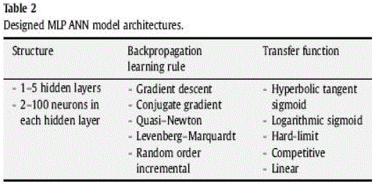where xmax and xmin are the expected maximum and minimum values of the concerned variable. x’max and x’min specify the desired values of the range for the transformed variable. After extensive simulations with all possible combinations of the 5 back propagation learning algorithms, the 5 transfer functions, the 1 to 5 hidden layers and the 2 to 100 neurons in each hidden layer, it was selected and used further to predict the energy consumption the model that presented the best generalizing ability, had a compact structure, a fast training process and consumed lower memory. This MLP ANN model had the following characteristics: 2 hidden layers, with 20 and 17 neurons in each one of them, Levenberg-Marquardt back propagation learning algorithm and logarithmic sigmoid transfer function. The mean square error was minimized to the final value of 0.010 within 13, 318 epochs.

Table 3 presents the training data of the best 10 designed ANN models which have presented the best generalizing ability among all the others designed.

TEST RESULTS – ERROR ANALYSIS

The selected ANN model has been used in order to predict the long-term energy consumption. Predictions have been made for years 2005–2008, 2010, 2012 and 2015. Table 4 presents the results produced by the developed ANN model and the real recorded energy consumption data/records for years 2005–2008.

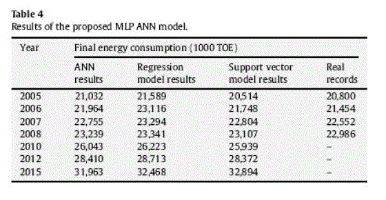In the same table are also shown the results produced using two other known methods obtained from technical literature in order to compare the accuracy of the developed method. The first method uses the linear regression model of equation (2).

where y is the final energy consumption, ai the regression coefficients (i= 0,1,2,3,4) estimated using a least square method, x1 is the yearly ambient temperature, x2 is the installed power capacity, x3 is the yearly per resident electricity consumption, x4 is the gross domestic product and e is the random error term.

The second method is based on the support vector machine model in which data is mapped into a higher dimensional feature space via non-linear mapping and then regression in this space is performed. The function of (3) is estimated based on the given data set G= [(xi,di)N i where xi is the inputs, di is the desired values and N is total number of data sets.

where Φi(x)is the set of mapping of inputs and wi and b are coefficients.They are estimated by minimizing the regularized risk function (4)

Where,

and ÃâÃâ is a prescribed parameter. It is obvious that the results obtained according to the proposed ANN method for the four known years (2005–2008) are close to the actual ones and comparable to these produced by the regression and support vector machine models.

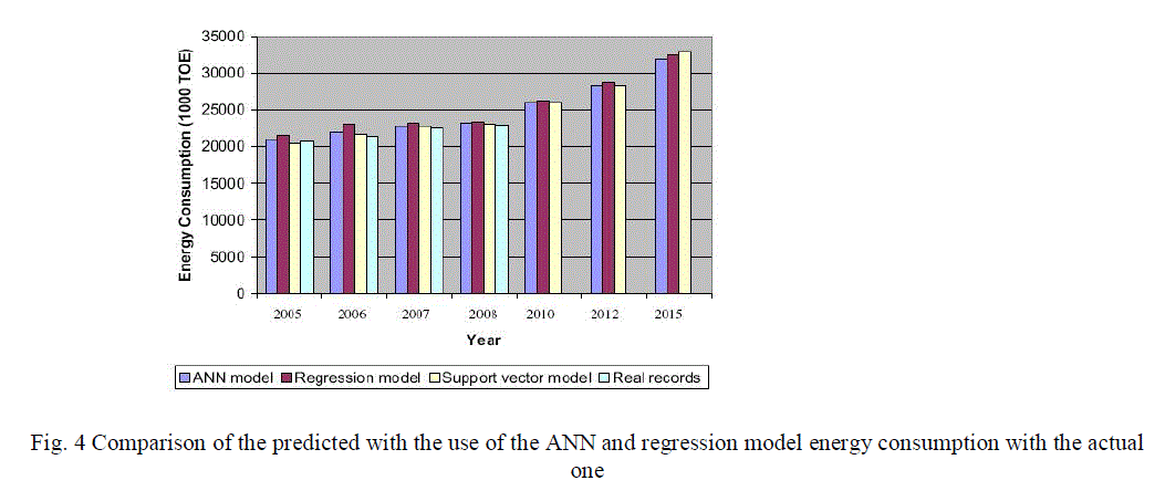
Fig. 4 presents the comparison of the obtained results with the actual recorded energy consumption data. The percentage error between recorded final energy consumption and ANN computed final energy consumption given by (6) is approximately 2% something which also clearly implies that the proposed ANN model is well working and has an acceptable accuracy.

where PE is the percentage error, FECrec is the recorded final energy consumption and FECcomp is the computed final energy consumption.

CONCLUSIONS

An artificial neural network method for the long-term prediction of Greek energy consumption has been described. Actual recorded input and output data which undoubtedly affect significantly the energy consumption were used in the training, validation and testing process. Predictions have been performed for years 2005–2008, 2010, 2012 and 2015 with the produced results to be close to the real ones, much more accurate than these obtained by a linear regression model and similar to these obtained by a support vector machine model. The proposed approach can be useful in the effective implementation of energy policies since accurate predictions of energy consumption affect the capital investment, them environmental quality, the revenue analysis, the market research management, while conserve at the same time the supply security. The evolvement of the produced ANN model in a user friendly software tool with the addition of a graphical user interface could constitute it an important tool in the studies of electric utilities and an accurate prediction for the country’s long-term energy consumption.

References

Sozen A, Arcaklioglu E, Ozkaymak M, “Turkey’s net energy consumption,”Applied Energy, 2005,Vol:81,pp:209–21.
Padmakumari K, Mohandas KP, Thiruvengadam S, “Long term distribution demand forecasting using neuro fuzzy computations,” Electrical Power and Energy Systems 1999,vol:21(5),pp: 315–22.
Mohamed Z, Bodger P, “Forecasting electricity consumption in New Zealand using economic and demographic variables,” Energy, 2005, vol:30, pp:1833–43.
Hsu CC, Chen CY, “Regional load forecasting in Twaiwan-applications of artificial neural networks,” Energy Conversion and Management, 2003, vol: 44, pp: 1941–9.
Haida T, Muto S, “Regression based peak load forecasting using a transformation technigue,” IEEE Transactions on Power Systems, 1994, vol: 9, pp: 1788–94.
Tso GKF, Yau KKW, “Predicting electricity energy consumption: a comparison of regression analysis, decision tree and neural network,” Energy, 2007, vol:32(9), pp:1761–8.
Hong WC, “Electric load forecasting by support vector model,” Applied Mathematical Modelling, 2009, vol: 33, pp: 2444–54.
Azadeh A, Ghaderi SF, Sohrabkhani S, “A simulated-based neural network algorithm for forecasting electrical energy consumption in Iran,” Energy Policy, 2008, vol: 36, pp: 2637–44.
Azadeh A, Ghaderi SF, Sohrabkhani S, “Annual electricity consumption forecasting by neural network in high energy consuming industrial sectors,” Energy Conversion and Management, 2008, vol:49, pp:2272–8.
Tay FEH, Cao LJ, “Modified support vector machines in financial time series forecasting,” Neurocomputing, 2002, vol: 48, pp: 847–61.