Evaluating the Effectiveness of Classification
Algorithms Based on CCI

R. Srujana; Dr. G S N Murty

Evaluating the Effectiveness of Classification Algorithms Based on CCI

R. Srujana ¹, Dr. G S N Murty ²

P.G. Student, Department of Computer Science and Engineering, Aditya Institute of Technology and Management, Tekkali, Srikakulam, India
Professor & Head, Department of Computer Science and Engineering, Aditya Institute of Technology and Management, Tekkali, Srikakulam, India

Related article at Pubmed, Scholar Google

Visit for more related articles at International Journal of Innovative Research in Science, Engineering and Technology

Abstract

Machine Learning has been widely applied to various domains and has gained a lot of success. At present, various learning algorithms are available, still facing difficulties in choosing the best methods that can be applied to their data. In this paper we perform an empirical study on 9 individual learning algorithms on a dataset by analyzing their performances and provide some Rules-of-thumb on selecting the algorithm over the dataset. To evaluate the performance, here we suggested supervised learning algorithm which can compute faster and better over the defined set of algorithms based on Time Complexity and Confusion Matrix. To assess the results over the given dataset, Receiver Operating Characteristic (ROC) curve is plotted on a graph by sensitivity or recall. Finally, a structured way to evaluate the performance of supervised learning algorithms is proposed, as well as suggested which algorithm is best suitable for their data set by comparing the effectiveness of various algorithms.

Keywords

supervised learning, Confusion matrix, ROC.

INTRODUCTION

Machine learning refers to a system that has a capability to automatically learn knowledge from experience and other ways. Classification and prediction are two forms of data analysis that can be used to extract models describing important data classes. The key question when dealing with machine learning classification is not whether a learning algorithm is superior to others, but under which conditions a particular method can be significantly outperform others on a given application problem [1][2]. So here we considered various classification algorithms on a dataset by evaluating their performance basing on some factors.

Given any existing implementation of a classifier learning algorithm for evaluation, weka API operates. However, respective users have to acquire a fairly deep knowledge in their dataset before adding learning algorithms implementation into them. Our MLEditor aims to fill this gap by providing an easy to use plug-and-play classifier assessment solution for the practitioner. Now-a-days, varieties of learning algorithms currently available for the researchers are enormous [1]. The main problems faced by the researchers are (i) How does one choose which algorithms is best suitable for the dataset? (ii) How does one compare the effectiveness of the particular algorithm to the others? The objective of this study is to provide some suggestions for the community by evaluating the Time complexity and confusion matrix of these classification learning algorithms. These two factors lead to obtain better and efficient results. This paper is organized as follows. Section 2 presents Background, Section 3 Classification algorithms, Section 4 dataset, Section 5 Evaluation, Section 6 Implementation Section 7, Results and the final section summarizes this work.

BACKGROUND

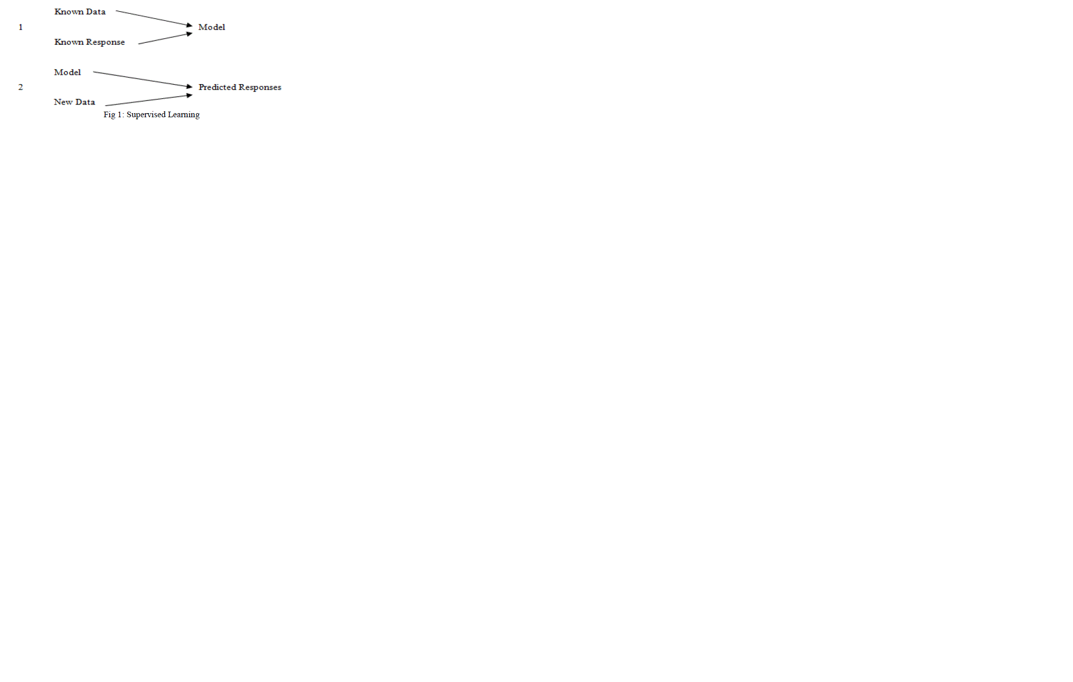
A machine learning algorithm is one that can learn from experience (observed examples) with respect to some class of tasks and a performance measure. These methods are suitable on various datasets due to the learning algorithm‟s ability to construct classifiers/hypotheses that can explain complex relationships in the data. Example applications include spam filtering, optical character recognition (OCR), search engines and computer vision. Machine learning is sometimes conflated with, and sometimes distinguished from data mining and pattern recognition [1][2][3]. Generally Machine learning tasks can be of several forms as supervised and unsupervised learning: Supervised learning takes a known set of input data and known responses to the data, and seeks to build a predictor model that generates reasonable predictions for the response to new data; and Unsupervised learning useful structure without labelled classes, optimization criterion, feedback signal, or any other information beyond the raw data. The overall tasks for the learner are to classify and characterize the input data. Supervised machine learning techniques are applicable in numerous domains like bio informatics, disease detection etc.

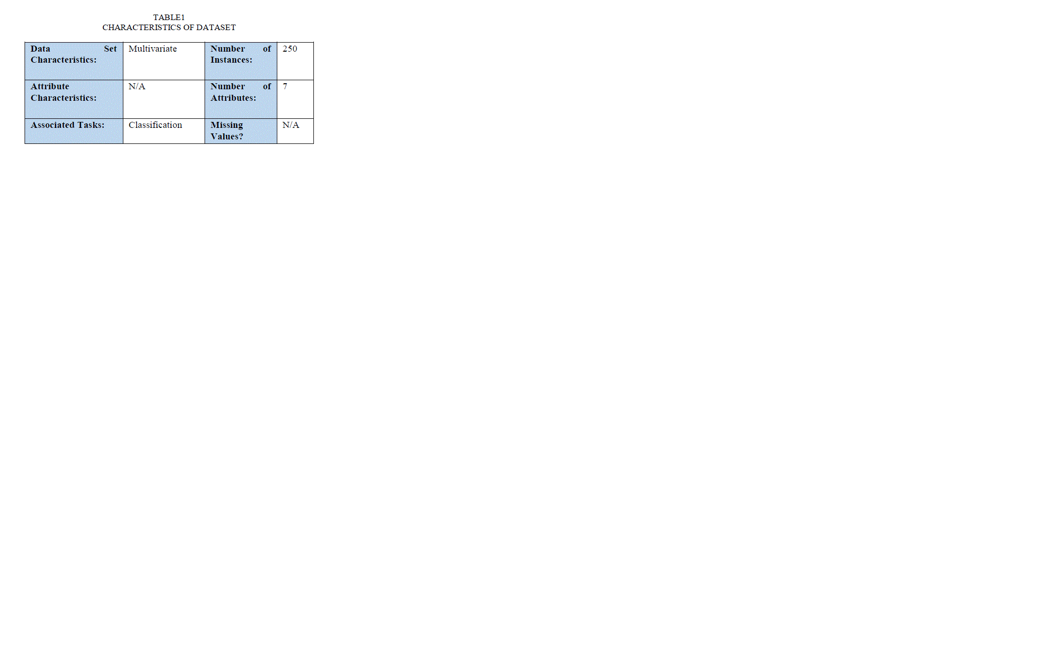
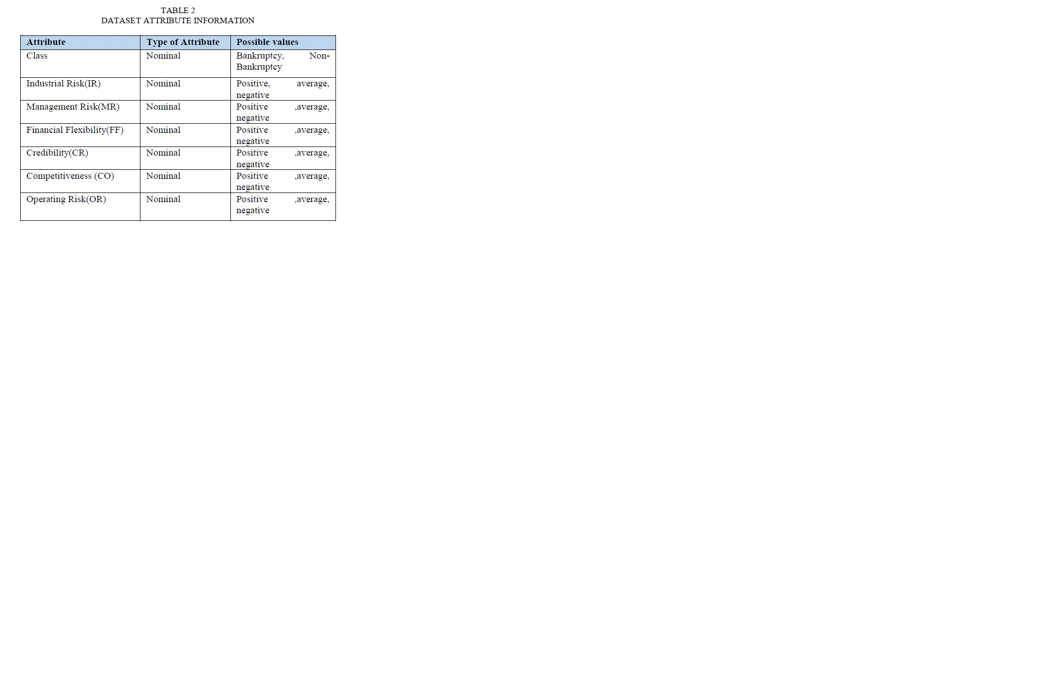
For the classification we are using BAYES NET, NAIVE BAYES CLASSIFIER, CONJUCTIVE RULE, DTNB (Combining Naive Bayes and Decision Tables), DECISION TABLE, OneR, JRip, NNge algorithms. Here we consider Multivariate dataset which is named as Qualitative Bankruptcy Data Set. Usually, for a supervised classification problem, the training examples are in the form of a set of tuples {(x1, y1j)…. (xn, ynj)} Where xi is the class label and yij is the set of attributes for the instances. The task of the learning algorithm is to produce a classifier (hypothesis, function) to classify the instances into the correct class. In this study, we only consider supervised machine learning applied to classification.

CLASSIFICATION ALGORITHMS

Here we used various algorithms for analysing dataset. Our approach is to identify an optimized algorithm which can perform better and analysis faster. All the learning methods used in this study were obtained from the WEKA machine learning package (http://www.cs.waikato.ac.nz/~ml/weka/)

BAYES NET: Bayes Nets or Bayesian networks are graphical representation for probabilistic relationships among a set of random variables. Given a finite set X=(X1,…, Xn) of discrete random variables where each variable Xi may take values from a finite set, denoted by Val (Xi)[2]. A Bayesian network is an annotated directed acyclic graph (DAG)G that encodes a joint probability distribution over X. The nodes of the graph correspond to the random variables X1… Xn. The links of the graph correspond to the direct influence from one variable to the other. If there is a directed link from variable Xi to variable Xj, variable Xi will be a parent of variable Xj. Each node is annotated with a conditional probability distribution (CPD) that represents p (Xi| Pa (Xi)), where Pa (Xi) denotes the parents of Xi in G. The pair (G, CPD) encodes the joint distribution p(X1,…,Xn). A unique joint probability distribution over X from G is factorized as:

p(X1,…,Xn) = Πi(p(Xi | Pa(Xi)))

NAIVE BAYES CLASSIFIER: A naive Bayesian network is a simple probabilistic classifier based on applying Bayes' theorem with strong independence assumptions [2]. Thus, the independence model is based on estimating:

Comparing these two probabilities, the larger probability indicates that the class label value that is more likely to be the actual label (if R>1: predict i, else predict j). Since the Bayes classification algorithm uses a product operation to compute the probabilities P(X, i), it is especially prone to being unduly impacted by probabilities of 0. The major advantage of the naive Bayes classifier is its short computational time for training.

DECISION TABLE: The simplest way of representing the output from machine learning is to put it in the same form as the input. It summarizes the dataset with a „decision table‟ which contains the same number of attributes as the original dataset [8]. Two variants of decision table classifiers are available. They are DTMaj (Decision Table Majority) and DTLoc (Decision Table Local).

DTNB: This is for building and using a decision table/naive bayes. The algorithm estimates the value of dividing the attributes into two disjoint subsets: one for the decision table, and the other for naïve Bayes [8]. The algorithm for learning the combined model (DTNB) proceeds in much the same way as the one for stand-alone DTs. The class probability estimates of the DT and NB must be combined to generate overall class probability estimates. The overall class probability is computed as

Q (y|X) = α× QDT (y|X>) × QNB (y|X⊥)/Q(y)

Where QDT(y | X>) and QNB(y | X ⊥) are the class probability estimates obtained from the DT and NB respectively, α is a normalization constant, and Q(y) is the prior probability of the class.

CONJUCTIVE RULE: Conjuctive Rule algorithm implements a single conjunctive rule learner that can predict for numeric and nominal class labels. A rule consists of antecedents “AND”ed together and the consequent (class value) for the classification or regression. In this case, the consequent is the distribution of the available classes (or mean for a numeric value) in the dataset.

OneR: The OneR algorithm creates a single rule for each attribute of training data and then picks up the rule with the least error rate [8]. To create a rule for an attribute, the most frequent class for each attribute value must be determined. The most frequent class is simply the class that appears most often for that attribute value.

JRip: JRip implements a propositional rule learner, Repeated Incremental Pruning to Produce Error Reduction (RIPPER). It is based in association rules with reduced error pruning (REP), a very common and effective technique found in decision tree algorithms.

NNge: Nearest-neighbour-like algorithm using non-nested generalized exemplars (NNge) (which are hyper rectangles that can be viewed as if-then rules).

PART: PART is separate-and-conquer rule learning. The algorithm producing sets of rules called „decision lists‟ which are ordered set of rules. A new data is compared to each rule in the list in turn, and the item is assigned the category of the first matching rule. The algorithm is a combination of C4.5 and RIPPER rule learning.

DATASET

In this study we used the following datasets from UCI Machine Learning Repository. We briefly describe the Qualitative Bankruptcy dataset [4]. Bankruptcy is financial failure of a business and when an organization not able to pay its debts is called as bankruptcy.

EVALUATION

A. Confusion Matrix:

In the field of machine learning, a Confusion Matrix, also known as a contingency table or an error matrix, is a specific table layout that allows visualization of the performance of an algorithm [6]. Each column of the matrix represents the instances in a predicted class, while each row represents the instances in an actual class. The below Table 3 with two rows and two columns reports the number of false positives (FP), false negatives (FN), true positives (TP), and true negatives (TN). This also allows more detailed analysis than mere proportion of correct guesses (accuracy).

To evaluate the performance and to measure the proportion of correctly classified instances (CCI) we use classifier accuracy in classification learning;

ACC= (TP+TN) / (TP+TN+FP+FN)

B. ROC

Receiver Operating Characteristics (ROC) graphs is a useful technique for organizing classifiers and visualizing their performance [7]. It is created by plotting the fraction of true positives out of the total actual positives (TPR = true positive rate) vs. the fraction of false positives out of the total actual negatives (FPR = false positive rate), at various threshold settings. TPR is also known as sensitivity or recall.

TPC= TP/P = TP/ (TP + FN)

The FPR is also known as the fall-out and can be calculated as one minus the more well-known specificity.

SPC=TN/N=TN/ (FP+TN)

FPR=FP/N=FP/ (FP+TN) =1-SPC

C. Time complexity

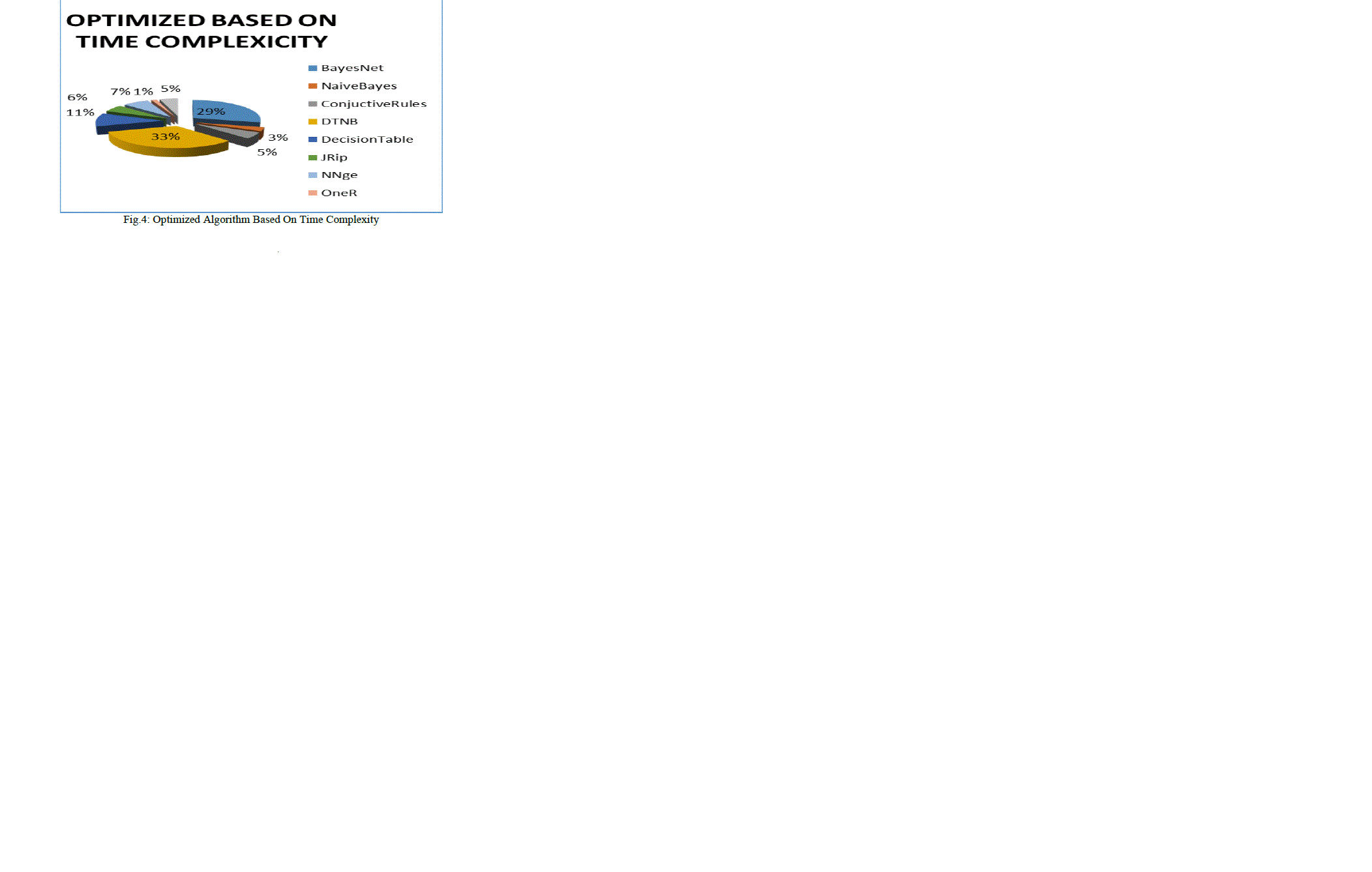
It is used to calculate the computational time. Here in this case we calculated time complexity among classification learning algorithm. Each algorithm is evaluated and obtained their burst time. Algorithm with least burst time on the dataset is the best algorithm to classify.

IMPLEMENTATION

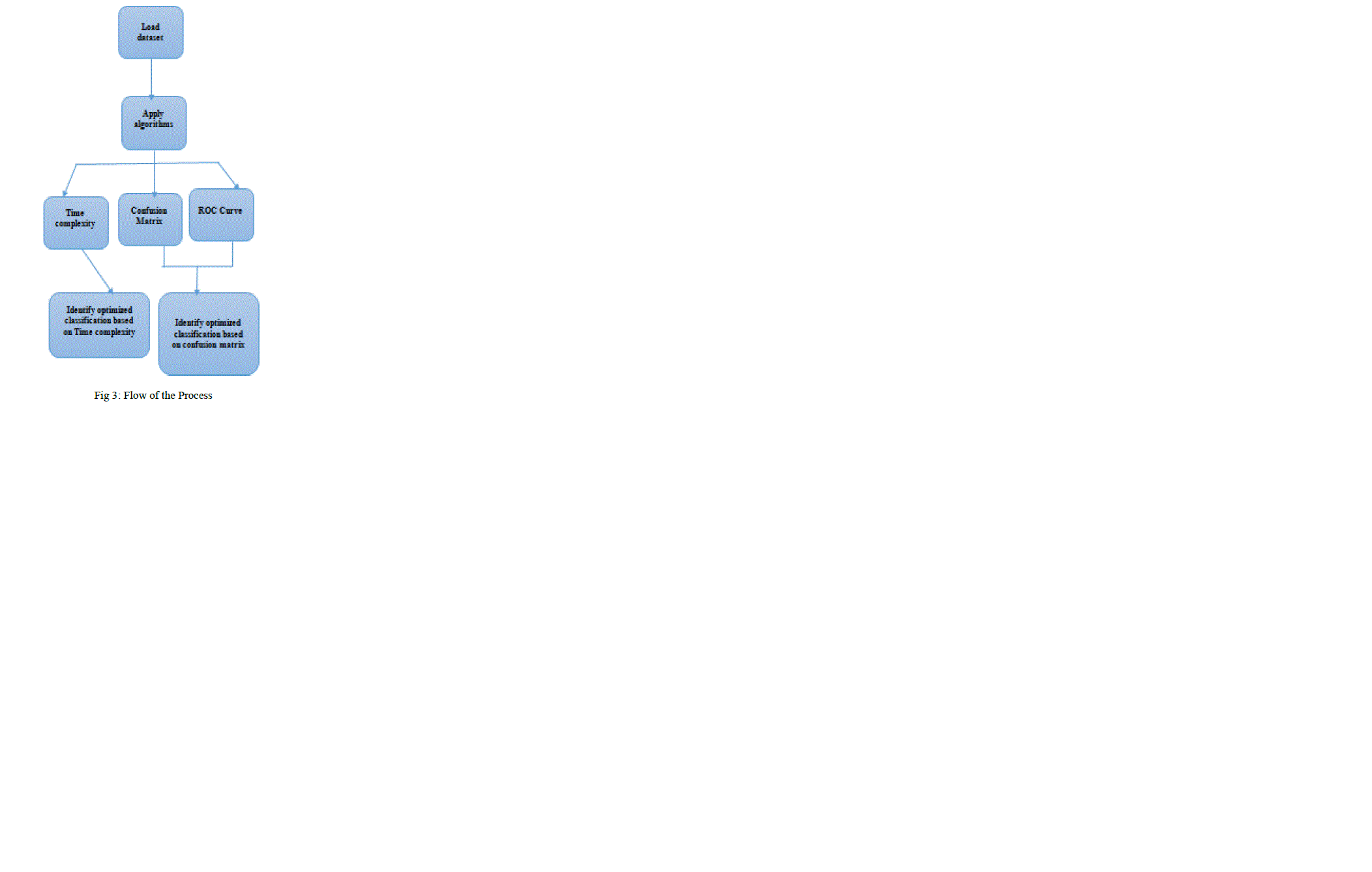
On computing the given dataset by using the classification algorithms, identified an optimized algorithm which can perform faster based on two factors i.e., time complexity and confusion matrix. Steps involved in the process:

1) Load dataset: The data set is initially available as an excel sheet. This sheet is converted in to an attribute relation file format (arff) which is the standard file format for data mining algorithms. Here we use a java program to load the dataset.

2) Apply algorithms: After the data set is loaded we use the following classification algorithms listed in section 3. On applying, calculates Time Complexity, Correctly Classified Tuples Percentage and ROC by Sensitivity or Recall.

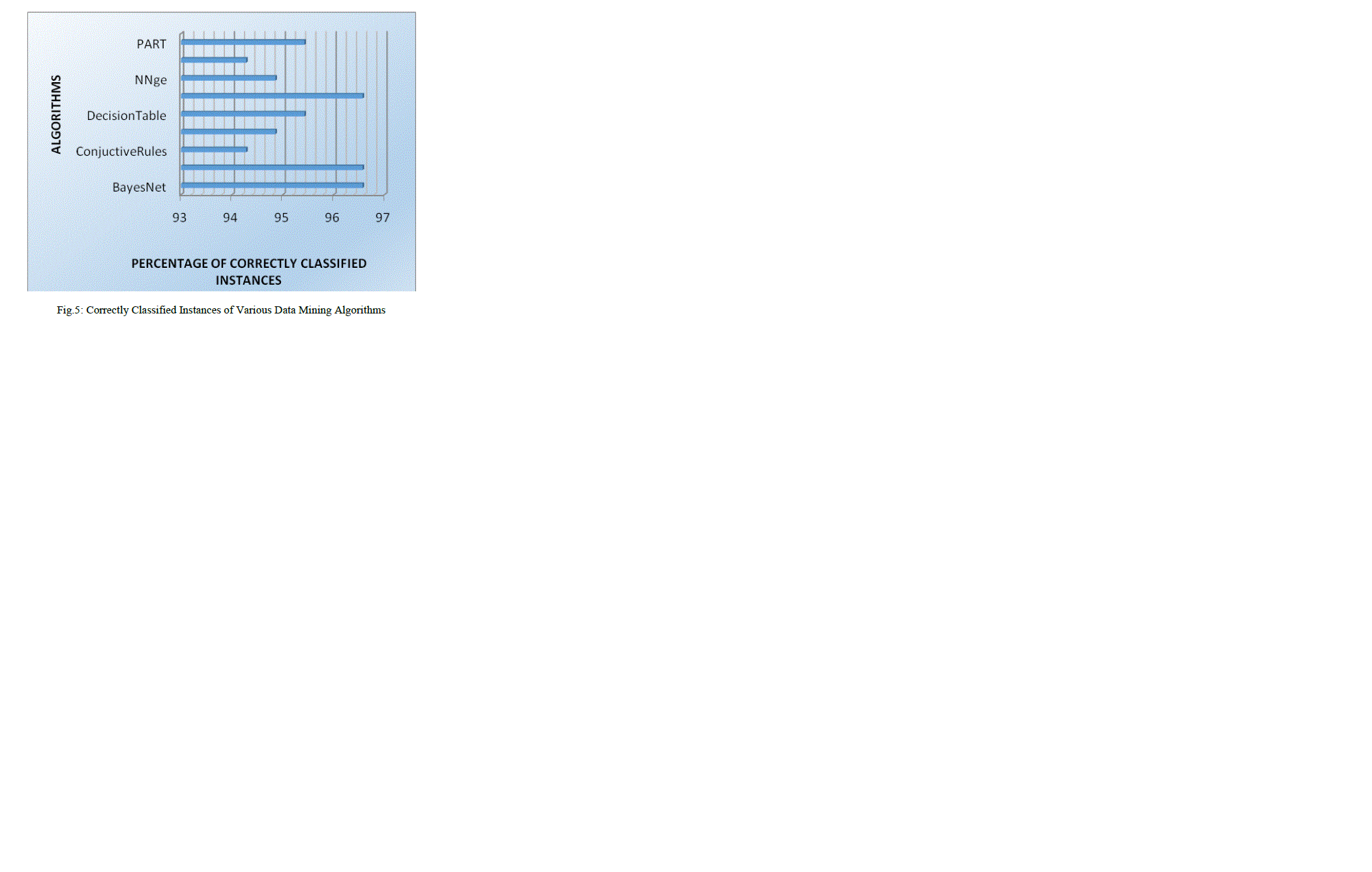
3) Identification of Optimized Algorithm: After completion of step2 we generate contingency matrix for each algorithm and comparison is performed among percentages of correctly classified instances to choose the better algorithm over given dataset. Even calculating the time complexity, best algorithm can be chosen over the given dataset.

RESULTS

From the results obtained the performance for various classification algorithms are shown below in graphical representation, which evaluated based on Time complexity and percentage of correctly classified instances.

SUMMARY

Machine learning has increasingly gained attention in various domains. On the availability of various learning algorithms, it has become common to apply the off-shelf systems to classify the datasets. Here in this paper we performed comparisons on various algorithms to classify. If we are interested in the best possible accuracy, it might be difficult or impossible to find a single classifier that performs as well as good ensemble of classifiers. Despite, we have shown how to choose which algorithms is best suitable for the dataset and how to compare the effectiveness of the particular algorithm to the others, on analyzing the Time Complexity and Percentage of Correctly Classified Instances. As Machine learning tasks can be of several forms as supervised and unsupervised learning. In future work we can apply an unsupervised learning on the dataset to analyse the performances.

ACKNOWLEDGEMENT

Authors are highly indebted to Director Prof. V.V. Nageswara Rao and Principal Dr. K.B. Madhu Sahu for providing excellent infrastructure facilities to accomplish this work. Authors would like to express their sincere thanks to Smt.N.Preeti, Asst.Prof Department of MCA, Aditya Institute of Technology and Management, Tekkali-532201, Srikakulam (dt), A.P.,for advising in manuscript preparation and for valuable suggestions and encouragement.

References

Aik Choon TAN and David GILBERT, An empirical comparison of supervised machine learning techniques in bioinformatics, International Journal of Information Technology Convergence and Services (IJITCS) Vol.1, No.4, August 2011.
S. B. Kotsiantis, Supervised Machine Learning: A Review of Classification Techniques, Informatica 31 (2007) 249-268 249
Dr. Mohd Fauzi bin Othman, Thomas Moh Shan Yau, Comparison of Different Classification Techniques Using WEKA for Breast Cancer, International Conference on Biomedical Engineering 2006.IFMBE Proceedings Volume 15, 2007, pp 520-523.
Myoung-Jong Kim*, Ingoo Han, The discovery of experts‟ decision rules from qualitative bankruptcy data using genetic algorithms, Expert Systems with Applications 25 (2003) 637–646.
Eibe Frank, Ian H. Witten, Generating Accurate Rule Sets Without Global Optimization, Fifteenth International Conference on Machine Learning, 144-151, 1998.
Using the confusion matrix for improving ensemble classifiers, Electrical and Electronics Engineers in Israel (IEEEI), 2010 IEEE 26th Convention of Date of Conference: 17-20 ov. 2010,Page(s):000555 – 000559
Tom Fawcett ,ROC Graphs: Notes and Practical Considerations for Researchers, HP Laboratories, MS 1143, 1501 Page Mill Road, Palo Alto, CA 94304,March 16, 2004.
S. Vijayarani, M. Muthulakshmi, Evaluating the efficiency of rule techniques for file classification, IJRET, eISSN: 2319-1163 | pISSN: 2321- 7308