ISSN ONLINE(2319-8753)PRINT(2347-6710)
ISSN ONLINE(2319-8753)PRINT(2347-6710)
Islam Sallam1, Ali Al-Nuaimi2, Ahmad Jamrah3
|
| Related article at Pubmed, Scholar Google |
Visit for more related articles at International Journal of Innovative Research in Science, Engineering and Technology
As population pressure in most of the world's regions increase, the demand for natural resourcesrises. Countries' strategies to deal with natural resources shortages depend on local conditions, including topography, the extent of resources scarcity, available financial incomes, and technical and institutional capacity. Overall, developing a mix of strategies that increase supply, manage demand, and reduce long-term pressures on natural resources is urgent more than ever before, as world’s population pressures continue to rise.This paper is exploring the relationship between the supply needs for a number of populations within a timeline frame in order to reach a balanced point that achieves the sustainable use of natural resources. The study creates an innovative approach that combines and modifies two well-known mathematical models. The first is Lotka- VolterraModel which is a non-linear, differential equations regularly used to describe the dynamics of biological systems in which two species interrelate, one a predator and one its prey. The approach was first created by Alfred J.Lotka, 1925, and modified statistically by Vito Volterra, 1926.The second Model is known as Supply and Demand Model which has been set by David Ricardo based on the influence of demand and supply on price.
Keywords |
| Sustainable Communities, Differential Equations, Biological Monitoring Systems, Supply and Demand, Mathematical Modeling. |
I. INTRODUCTION |
| Many arguments have been made to investigate the factors that affect urban settlements and their ability to comply with sustainable development plans. Of these factors, the Natural Resources (NR) is one of the most important elements that play an essential role in the evolution and continuity of those settlements. The idea of sustainable development is not to think about the problems and shortages presently, it is how much the community is ready to accomplish future generation's needs. It is a matter of scientific prediction that this paper is outlining as a benchmarking indicator of equilibrium state which conserves and sustains a certain (NR) volume against the population increasing demands. |
| To face the unrestrained population growth and its effect on planet's (NR), a new concept was set to face and control this problem known as Sustainable Urban Settlements (SUS). With all respect to this concept, it lacks a crucial indicator which is the determination of population max-size that can sustain the available (NR); or in other words, it lacks a precise scheme that clearly identified the behaviour between population size (W) and obtainable natural resource (NR). |
| The behaviours of such schemes have been viewed in three particularly different ways in literature. The first early models claimed that such systems obtain a stable equilibrium point. It is conceivable to detect random shocks, but eventually equilibrium would always be restored. Later models presumed that growth paths are cyclical and any equilibrium or balance is affected by past indications. Since the commencement of modern statistical techniques, it has been assumed that random shocks create what can fundamentally be seen as chaotic behaviour. |
II. AIMS AND OBJECTIVES |
| The main aim of the paper is to find: |
| a) The relationship between population number W and natural resource R volume in a certain location within defined time; |
| b) Define the equilibrium point when the R volume reaches its critical point to support a given number of W. The study used a system of differential equations to create a mathematical model capable to achieve its goals. |
III. CREATING A MODEL |
 |
| This was effectively the logistic formula,[4] which was originally presented by PierreFrançois Verhulst. In 1920 Lotka lengthened, via Kolmogorov, the formula to "Organic Systems" using a plant species and a herbivorous animal species as a model[5] and in 1925 he developed the equations to examine predator-prey interactions in his book on biomathematics [6] inward the equations to the its nowadays well-known shape. Vito Volterra, who made a statistical analysis of fish catches in the Adriatic Sea [7] independently investigated the equations in 1926.[8][9] |
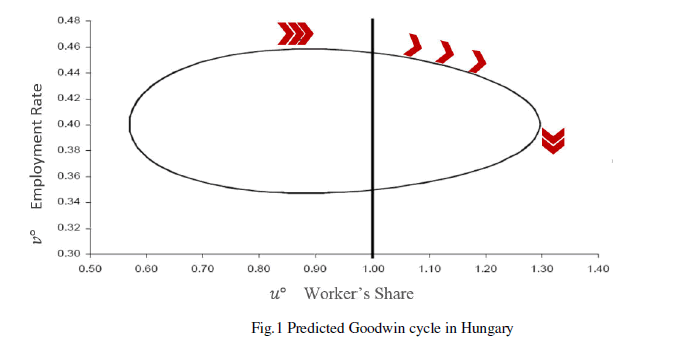
| C.S. Holling comprehensively widened this model in two papers in 1959, in which he anticipated the idea of functional response. [10][11] Both Lotka-Volterra model and Holling's additions have been used to prototype the moose and wolf populations in Isle Royale National Park, [12] which with over 50 published papers is considered one of the best studies that analyzed predator-prey relationships. In economics, the Lotka–Volterra equations have a long history of use in economic theory; their early application is generally credited to Richard Goodwin in 1965[13] or 1967.[14][15] Moreover, links between many if not all industries were proposed to prototype the dynamics of many businesses by introducing trophic functions between sectors,[16] with disregarding smaller sectors by considering the collaborations of only two industrial/ businesses sectors. [17] In the original Lotka-Volterra model of opposing kinds of bio systems, the predator and the prey can be classified by the fact that the predator population breeds faster the higher the prey population is, though the prey population breeds faster the lesser the predator population is. Goodwin acknowledged u with workers’ share while 1-u is capitalists’ share of output and v is the employment rate. |
 |
| From equation {γ}, the employment rate increases more rapidly the larger the businesspersons’ share, and from equation {4}, the businesspersons’ share increases more rapidly the smaller the employment rate is. In this model of Goodwin, employees are the predators and businesspersons are the prey. The economic suggestion of this relationship is relatively simple. When incomes are high, investment is high, and because all investment needs additional employment, high investment interprets into a fast employment progression. On the other hand, when employment is low, salaries are decreasing and, in turn, incomes rise as can be concluded from figure 1. |
 |
| Accordingly, and based on the previous interpretation, the similarity is purely proper, but not totally so. It has long seemed that Volterra’s problem of such interaction of two populations partly complementary, partly hostile, but is helpful in the understanding of the interaction between two competing variables. From a mathematical standpoint, this similarity can introduce solutions for such complicated looking system immensely easier. |
| B. Justifying the proposed model |
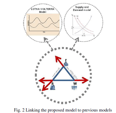
| By considering population as a predator or a demand (consumers); and natural resource as a prey or a supply (consumed), then, the question that may be derived can be formulated as: “Can a model that take into account the correlation between population and natural resource in a certain location, take the same form of interaction?”The Lotka-Volterra model makes a number of rules about the environment and growth of the predator and prey populations. As differential equations are used, the solution is deterministic and continuous. Consecutively, implies that the groups of both the predator and prey are repetitively overlapping. [18] |
 |
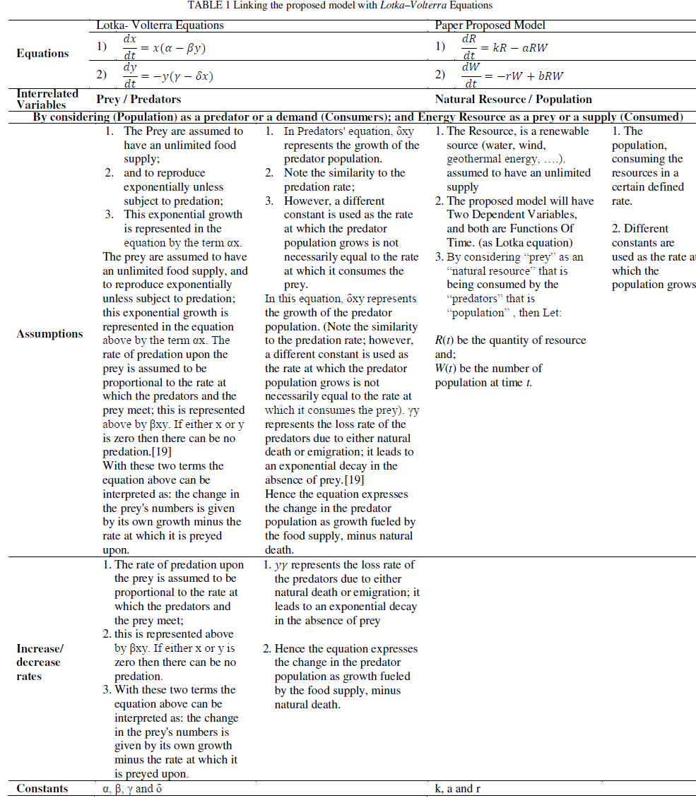 |
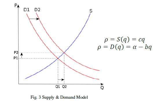
| For more validation and to draw some similarity evidences that can link our case with Lotka-Volterra equations and Supply & Demand Model, the paper proposed model includes: |
| a. The three Models are dealing with three matching variables; time t, consumed entity R and a consumer W. |
| b. They are using fixed/ flexible constants according to time, number of consumers and rate of consumption |
| c. The proposed model and the equations of Lotka-Volterra have periodic solutions and do not have asimple expression in terms of the usual trigonometric functions. However, a linearization of the equations yields a solution similar to simple harmonic motion with the number of consumers following that of consumed object by 90°. |
| d. The proposed model and Supply & Demand Model are following four basic rules |
| o Demand increases (leads to higher price and quantity). |
| o Demand decreases (leads to lower price and quantity). |
| o Supply increases (leads to lower price and higher quantity). |
| o Supply decreases (leads to higher price and lower quantity). |
 |
| C. Tapping into creating a new model |
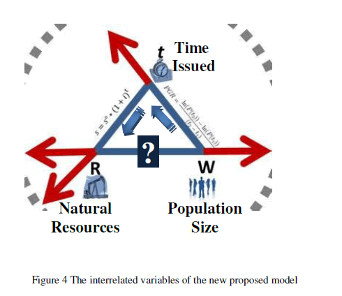
| The study sets three variable to be tested through its model; Population W, Natural Resources R and Time t. |
 |
 |
 |
 |
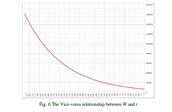 |
| From the previous equation; it can be concluded that there is a vice-versa relationship between those two variables. The more time passed the more population we have according to(r) the population growth rate. (in normal circumstances) |
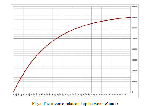
| - The final relationship is between (R) and (W). Logically it can be concluded that there is an inverse relationship between the two variables. The more population you have the more decrease in natural resources amount you get. But the issue here is different; the study is trying to find out the balance between those two variables; the equilibrium point in another words that always maintain a sufficient level of R capable to sustain population in a certain community; now and in the future. |
IV. MODIFYING LOTKA-VOLTERRA EQUATIONS |
| Lotka-Volterra equations as previously stated are differential equations that can be used to model predator-prey interactions. The original system consisted of two entities. Vito Volterra developed these equations in order to model a situation where one type of entity is the prey for the other type. To implement the model on natural resources as the first entity while population represents the other; the proposed model was restrained by the following consideration: |
| A. Consideration |
| The considerations that should control the proposed model have an influence on the two main variables as; |
| o The R should be renewable (water, wind, geothermal energy…). |
| o The population W is consuming R in a certain defined rate. |
| o The proposed model’s two dependent variables are functions of time. (as Lotka equation) |
| By considering “prey” as R that is being consumed by the “predators” that is “population” W, then let: |
| o R(t) be the quantity of natural resource at time (t) and; |
| o W (t) be the number of population at time t. |
| Accordingly, there are two cases can be assumed: |
| Absence of population “predators” |
| In the absence of “Population”, the R supply would take the form, that is, |
 |
| Absence of natural resource R “prey” |
| In the absence of R, it can be assumed that the “Population” W would decline at a rate proportional to itself, that is, |
 |
| B. Assumptions |
| With both variables present, the assumption will be: |
| o The principal cause of resource declination is being consumed by a population of a certain location. |
| o The birth and survival rates of the population in a certain location depend on their available life support— namely, the resource. |
| o Also by assuming that the two variables encounter each other at a constant rate that is proportional to both population and resource quantity, therefore, proportional to RW. |
| A system of two differential equations that incorporates these assumptions will be: |
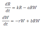 |
| Where k, r, a, and b are positive constants. Noting that the equations have slightly modified using “Chain Rule” based on the nature of the relationship between Population/Resource and Predator/Prey. |
| Noticing that |
| • The term –aRWdecreases the natural growth rate of the resource quantity. |
| • The term bRWincreases the natural growth rate of the population. |
| C. Solutions to the equations |
| A solution of this system of equations is a pair of functions R(t) and W(t) that describe the R amount and population of a certain community as functions of time. Thus: |
| As the system is coupled (R and W occur in both equations), equations can’t be solved separately. |
| They have to be solved simultaneously. |
| Unfortunately, it is usually impossible to find explicit formulas for R and W as functions of t. However, so graphical methods can be used to analyze these types of equations. By using the same principles of Lotka-Volterra equations, with the application of “Chain Rule”, the constants of the new equations will be: |
| k = 0.08, a = 0.001, r = 0.02, b = 0.00002 |
| The time t is measured in months. |
| One can also plot solutions without representing time, but with one axis representing the quantity of R and the other axis representing the number of population. |
V. POPULATION/RESOURCE EQUATIONS |
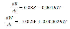
| Supposing that, at some point in time,there are 1000 units (mγ, liters, watt, …) of the energy resource and 40 units of population (40X10, 100, 1000, ……). With the given values of k, a, r, and b,the proposed “Population-Resource” equations become: |
 |
| A. Equations’ Probabilities |
Probability 1 |
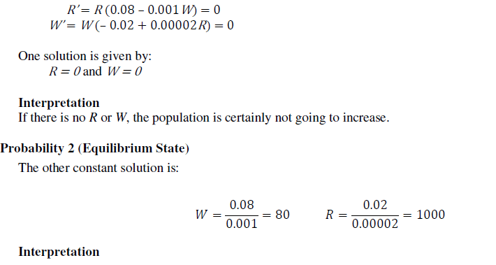
| Both R and W will be constant if both derivatives are 0. That is, |
 |
 |
 |
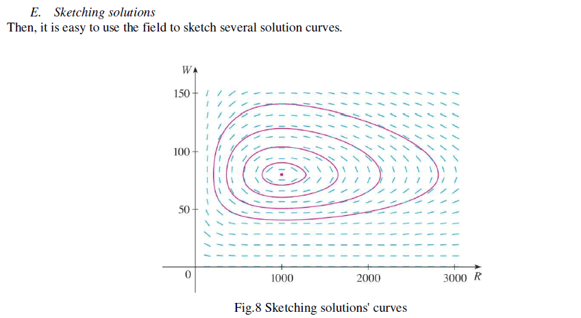 |
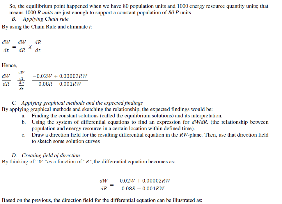
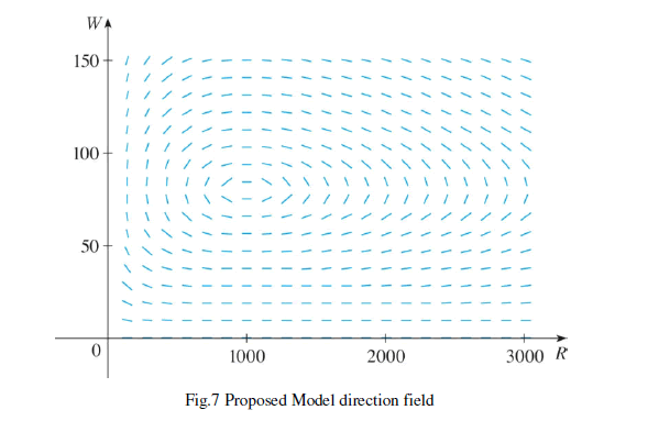
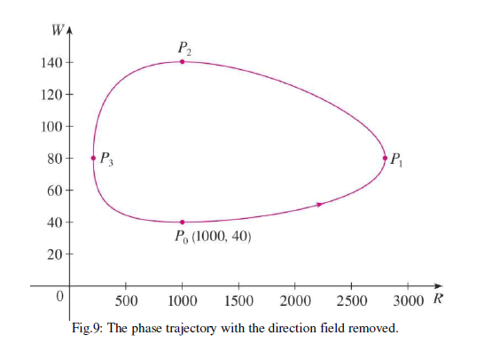
| By tracking points along the solution curve, it can be detected how the correlation between R and W changes as time passes. Noting that the curves seem to be closed in the sense that moving along the curve, will always return to the initial starting point. Noting also, that the point (1000, 80) is inside all the solution curves as it signifies an equilibrium point. It recounts the equilibrium solution R = 1000, W = 80 |
| When representing solutions of a system of differential equations as here, it is referred to the RW-plane as the phase plane. Accordingly, the solution curves are called phase trajectories. A phase trajectory is a path traced out by solutions (R, W) as time goes by. A phase portrait, as shown, consists of: |
| • Equilibrium points |
| • Typical phase trajectories |
| For example, starting with 1000 energy resource units and 40 population units (multible corresponds to drawing the solution curve through the point P0 (1000, 40). |
 |
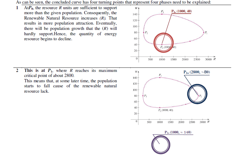
| F. Interpreting Curve Turning Points |
 |
 |
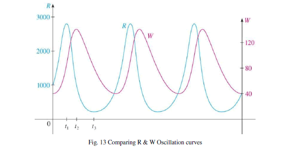 |
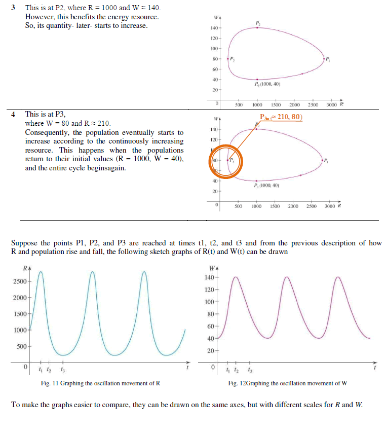
| It can be noticed from the previous chart that the energy “R” resource units reach its maximum quantity about a quarter of a cycle before the “W” population. |
| These graphs clearly illustrate a serious problem with this as a proposed model: in each cycle, the R is reduced to extremely low numbers yet recovers (while the W population remains sizeable at the lowest R density). With chance of oscillations, distinct numbers of individuals, and the family structure and lifecycle of W, the R actually go fade and consequently the W as well. This phenomenon appeared in previous similar studies that used Lotka-Volterraequations as a modeling system to describe the relationship between two or more biological systems and has been called the "atto-fox problem". [22] |
VI. THE BALANCE |
| In this model system, the W population thrive when there are plentiful R but, ultimately, outstrip their need supply and decline. As the W population is low the R amounts will increase again. These dynamics continue in a cycle of growth and decline. Population equilibrium or balance occurs in the model when neither of W population number nor the R amounts is changing, i.e. when both of the derivatives are equal to 0. |
 |
| Hence, there are two equilibrium points; |
| 1. The first effectually signifies the extinction of W and the fade of R. If both variables are at 0, then they will continue to be so indefinitely. |
| 2. The second solution signifies a fixed point at which both W and R sustain their current, non-zero numbers, and, in the simplified model, do so indefinitely. The number of W population at which this equilibrium is achieved depends on the chosen values of the parameters, k, a, b, and r. |
| The stability of the fixed point at the origin can be determined by performing a linearization using partial derivatives, while the other fixed point requires a slightly more sophisticated method. In the study of dynamical systems, linearization is a method for assessing the local stability of an equilibrium point of a system of nonlinear differential equations or discrete dynamical systems.[23] |
| In the model (k and r) are always greater than zero, and as such the sign of the two variables W and R above will always vary. Therefore the fixed point at the origin is a saddle point. |
| The stability of this fixed point is of importance. If it were stable, non-zero populations might be attracted towards it, and as such the dynamics of the system might lead towards the extinction of both variables for many cases of initial population levels.[24] However, as the fixed point at the origin is a saddle point, and hence unstable, the study finds that the extinction of both variables is difficult in the model. In fact, this can only occur if the R is artificially totally eliminated, causing the W population to fade of R scarcity. According to paper assumption of the renewable resource applied in the equations, so this case is almost impossible. If W is eradicated, the R amounts grow without bound in this simple model. |
| Evaluating W and R at the second fixed point we get purely imaginary values for both of them. This fixed point is not hyperbolic, so no conclusions can be drawn from the linear analysis. However, the system admits a constant of motion and the level curves, where k is constant, are closed trajectories surrounding the fixed point. Consequently, the levels of the population size W and renewable natural resource R cycle, and oscillate around this fixed point. |
VII. CONCLUSION |
| Natural resource management became an important focal point of modern sustainability concepts. Therefore measuring how social and economic systems are evolving to sustainability is a significant require. This paper claimed that this evolving or interaction is dependent on the improvement of analytical, methodological and mathematical models to measure and control progress, particularly, for sustainable communities. Achieving sustainability on the scale of maintaining natural resources is a key for social and ecological performance that are mostly closely linked to population size and type. Accordingly, the paper proposed a new mathematical model that is considered a modification of two well-known models; Lotka-Volterra Equations and Supply and Demand model. The paper developed and theoretically tested this new model for assessing the sustainability of natural resource by finding the equilibrium points that achieve balance between the population size and the available natural resources. The study believes that this model is applicable at the micro and regional scale. The proposed model evaluates and controls the interaction between human activities as a population size by considering them as predators consuming natural resources as preys which increase the pressures on regional ecosystems. The theoretical test applied signified its potential to be an effective method for monitoring the sustainability of natural resources. It also has potential ability to be employed as a community warning or for decision makers to guide them setting their strategic plans for sustainability improvement. |
References |
|