GIBBS ENSEMBLES MONTE CARLO SIMULATIONS OF PHASE EQUILIBRIA OF BINARY MIXTURES CONTAINING NITROGEN AND OXYGEN

Abstract

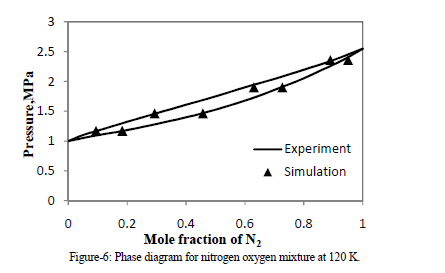
The NpT-Gibbs ensemble Monte Carlo computer simulation method is applied to predict the vapor-liquid equilibrium (VLE) behavior of binary system Nitrogen + Oxygen at 120 K. The Lennard-Jones potential is used to describe the interactions of Nitrogen and Oxygen mixture. The result show that the simulated values of densities of the pure components are within a few percent of corresponding experimental data. In addition, the simulated pressure composition diagram for a binary mixture of Nitrogen and Oxygen also shows satisfactory agreement with the experimental data.

Keywords

Gibbs ensemble, Monte Carlo, Molecular Parameters, Nitrogen and Oxygen, Vapor-liquid Equilibrium

INTRODUCTION

The most important part in modeling a process involving fluids is vapor-liquid phase behaviour. This importance creates a need for accurate equilibria data for Binary systems, which can be applied to various chemical processes. For instance, to successfully design any type of separation apparatus, system has to know how a Binary mixture is equilibrating. Over the years, various modeling techniques have been designed to describe Binary systems. The equation of state method is useful for simple fluids, but it has its drawbacks. It begins to run into problems for more complicated systems, such as aqueous systems at high pressures or ionic systems. Another limitation is that it relies on experimental data. Lastly, one can not extrapolate with confidence outside the range of experimental data. These problems create a need for a different methodology to find equilibrium data. Hopefully, this need can be filled be the technique of molecular simulations. It was not until recent developments that this method became practical to run on computers. A widely-used method for two-phase molecular simulations is the Gibbs ensemble Monte Carlo method [1]. This technique is used to find vapor-liquid equilibria data first for pure N2 and O2, and then for mixtures of these components. Then, the results are compared to experimental data. Finally, after finding the best parameters to fit the experimental data, runs are done to see how accurately the parameters predict the behavior of these systems at high density and pressure in the single phase.

II. MOLECULAR SIMULATION METHOD

A. Setting Up a Model

The first step in running a molecular simulation is making a model of the molecule or molecules is to used. In these simulations, the Lennard-Jones potential is used to calculate the energy of the interactions by Equation (1)

Uij(r) = 4 × εij [(σij/r) 12 - (σij/r) 6] (1)

Where U is the configurational energy of interaction between the centres of two beads i and j a distance r apart. εij and σij are energy and size parameters for the ij interaction. σ has units of length which represents the diameter of the bead. ε has units of energy, and represents the depth of the potential well. For interactions between different types of beads, the Lorentz-Berthelot combining rules are used by Equations (2) and (3).

σij = (σii + σjj) / 2 (2)

εij = (εii × εjj)1/2 (3)

This procedure can be expanded to describe a system made up of hundreds of diatomics. Although there are other models that describe actual intermolecular potential better, the Lennard-Jones model is much simpler and there is a lot of literature on its properties to use for comparison to simulations.

B. Running a Simulation

Before discussing the algorithm for doing the Gibbs ensemble calculation, let us look at the principle behind it. Figure 1 show a macroscopic two-phase region which is in equilibrium. The procedure is to be performed on a microscopic section in each of the regions. Thermodynamics gives the following requirements for equilibrium: each region is in internal equilibrium and the temperature, pressure, and chemical potential of all components in both phases are equal. First, we deal with the pure system case and then we move on to multi-component mixtures. Phase I is the gas phase and Phase II is the liquid phase. The pure system have constant temperature T, total volume V (= VI + VII), and total number of particles N (= NI + NII). For this reason it is referred to as a constant NVT system. In the pure component case, temperature is set before the simulation is performed. The other three thermodynamic requirements are satisfied by three types of moves (Figure 2): displacement of molecules within each region, volume changes of the two regions, and particle transfers between the regions. These moves satisfy internal equilibrium, equality of pressure and equality of chemical potentials respectively.

The simulation runs as follows. After entering in all the necessary parameters (temperature, number of particles initially in each phase, initial densities, epsilon, sigma, the bond lengths), the program starts by generating an initial configuration. Next, it picks a type of move to perform. The percentage of how often a move is picked is set by the user (example: 30% displacement, 1% volume change, 69% transfer). Then, the computer attempts to make that move. The probability of the move being accepted is calculated by one of the following formulas, where ptransfer is the formula for a transfer from region II to region I.

pdisplacement = min [1, exp (-β × Δ U)] (4)

pvolume = min [ 1 , exp(-β × Δ UI - β× ΔUII + NI ln ( VI + ΔV ) + NII ln ( VII - Δ V ) ] (5)

ptransfer = min [1, NII × VI / ((NI + 1) × VII) × exp (-β × Δ UI -β × Δ UII] (6)

The computer generates a random number between zero and one. If this number is greater than the probability, then the move is rejected and the system retains the old configuration and a new move is attempted. If it is less than or equal to the number than the move is accepted and the system moves to the new configuration. This cycle is repeated on the order of 106 times. There are two periods of the simulation - the equilibration and production periods. The simulation records certain properties of the system (pressure, density, internal energy) and averages them over the production period to use for the equilibrium data at that temperature. There is an upper and lower temperature limit that can be used for each system when the temperature is too low, the liquid phase begins to get very dense and the chemical potential equilibration is difficult to satisfy because most of transfer moves are rejected. A particle has trouble moving from gas to liquid because most of the attempted transfers place it in a position overlapping another particle. Moving a particle from liquid to gas is difficult because it involves a large cost in energy. The upper limit is the critical point. Once the temperature of the run gets too close to the critical point, the length of interaction between molecules approaches infinity.

III. RESULTS AND DISCUSSION

Molecular simulation Phase equilibrium data is obtained from [2].The molecular interaction parameter are given in table-I [3].The results section is divided into three parts - nitrogen, oxygen, and nitrogen-oxygen mixtures. Nitrogen covered in greater detail than oxygen, since the methods are repeated.

The formulas used to reduce the system are:

T* = T × kB/ε (7)

ρ*= ρ × (σ)3 (8)

P* = P × σ3/ε (9)

A. NITROGEN

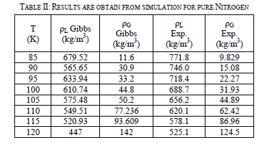
Eight runs are done for the pure nitrogen system from 85K to 120 K at 5 degree intervals using the Gibbs Ensemble Program. The parameters are given in Table-I, where kB is Boltzman’s constant: set up with densities of 500 kg/m3 and 50 kg/m3, respectively. The first two million steps of the simulation are used to equilibrate the system and the next are for the production period. In order to check that the system had equilibrated before the production period began, the density of both the liquid and vapor phase are plotted out Figure 3.

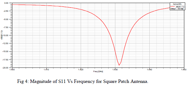
Table-II shown of the two-phase region results. After the runs are performed, they are compared to experimental data [4] in Figure 4. The graph is a little deceiving. At low temperatures, it appears that vapor simulation points overlap with the experimental points. On the liquid side, the simulation under predicts the density at lower temperatures until 100 K. Over 100 K, it begins to over predict the density of the liquid. Another interesting property the Gibbs Ensemble Program calculates is the pressure of the boxes. The tests for the validity of these new Lennard-Jones parameters are to see how they predicted system behaviour at high pressures and densities. NVT simulations are run with 512 particles in a box. This kept the density constant while the pressure of system is calculated. Runs are done at various densities at 120, 130, and 150 K. The simulation results are accurate at lower densities, but starting around 600 kg/m3 the simulation began predicting higher pressures than actual experimental results show. Around 800 kg/m3, the simulation had trouble creating a starting configuration, so NVT runs above this point are not done for nitrogen (not shown here).

B. OXYGEN

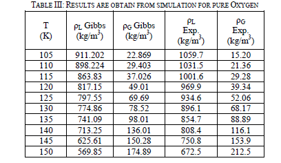
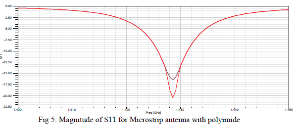
Eleven runs are performed for pure oxygen from 105 K to 150 K at 5 degree intervals using the Gibbs ensemble program. The run at 100 K is unsuccessful due to a shortage of phase transfers. It is not used in the analysis of the data. The runs are performed up to 150 K because oxygen has a critical point of 154.77 K. The liquid and vapor phases are initially set up with densities of 900 kg/m3 and 50 kg/m3, respectively. As in the nitrogen simulations, there are two million equilibration and the next are production steps. Table-III shown of the two-phase region results. After the runs are performed, they are compared to experimental data [5] in Figure 5. The analysis performed on oxygen is the same as the one on nitrogen. Once again, the simulation data correctly predicted experimental behaviour at lower temperatures on the vapor side, but under predicted for the liquid density and over predicted higher temperature vapor density.

C.NITROGEN-OXYGEN MIXTURES

Four NPT runs of different mixtures of nitrogen and oxygen are performed. Mole fraction data of vapor and liquid for N2 obtain from molecular simulation are match with experimental VLE data [6] of N2 + O2 at 120 K. By simulation, an equimolar composition in the liquid phase was regarded, where the mixing effect is strongest.

IV. CONCLUDING REMARKS

Nitrogen and oxygen binary mixture is cryogenic system it means mixture has to be very low temperature and the vapor liquid equilibrium data obtain from simulation are match with the experimental data. From this molecular simulation method it is possible to obtain vapor liquid equilibrium data for very low temperature system which is not possible by experiment.

References

1. Panagiotopoulos, A.Z., "Direct determination of phase coexistence properties of fluids by Monte Carlo simulation in a new ensemble", Molecular Physics., vol.61,pp.813-826, 1987.
2. Patel S., “Molecular Simulation of Phase Equilibria using Monte Carlo Simulation”, M.Tech. Thesis, M.S.University, Baroda, 2010.
3. Mulero A, Larrey D and Cuadros F., “A new correlation for VLE data: Application to binary mixtures containing nitrogen”, Korean J. Chem. Eng., vol.23(4), pp.650-657, 2006.
4. IUPAC, table 4, vol.6,pp.230-232, 1963.
5. Handbook of Physical Properties of Liqids and Gases Second Edition, Chapter 6, N.B. Vargaftik Hemishphere Publishing Corp.,1975.
6. Dodge BF, Dunbar AK. “An investigation of the co-existing liquid and vapor phases of solutions of oxygen and nitrogen”. J Am Chem Soc., vol.49(3), pp.591–610, 1927