Data mining is the domain which has utility in real world applications. Data sets are prepared from regular transactional databases for the purpose of data mining. A huge amount of time is needed for making the dataset for the data mining analysis because data mining practitioners required to write complex SQL queries and many tables are to be joined to get the aggregated result. We recommend simple, however powerful, techniques to generate SQL code to return aggregated columns in a very horizontal tabular page layout, returning a few numbers as opposed to one variety per short period. This new class involving functions is named horizontal aggregations. Horizontal aggregations build data sets with a horizontal denormalized layout (e.g., point-dimension, observation- variable, instance-feature), which is the standard layout required by most data mining algorithms. This paper focuses on building user-defined horizontal aggregations such as PIVOT, SPJ (SELECT PROJECT JOIN) and CASE whose underlying logic uses SQL queries, which prepares a query set consists of procedures and this query set will be stored in the database. One can easily access the query set and get the desired output to analyze the datasets. The queries which are not available in the query set can be generated dynamically using dynamic query generation. Finally we will see the experimental evaluation of data sets using SPJ and CASE method.
Keywords |
| Data Mining, Horizontal Aggregations, PIVOT, SQL, CASE, Data Sets, Query Sets, Dynamic Query. |
I. INTRODUCTION |
| Database model such as RDBMS has been used widely for storing and retrieving real world business data. Though the
databases support mechanism for data storage and retrieval, they are used in data to day operations. For making well
informed business decisions, it is essential to mine such data to extract trends or patterns from the data. However,
transactional database cannot be used directly for data mining. Therefore preparing datasets for data mining purposes
assumes significance. However, the existing aggregation functions available in SQL do not support to generate datasets
as they can only produce single row outputs. The summary of business data can be given for data mining purposes
instead of giving the whole business data. |
| This is the idea behind preparing datasets for data mining. As the vertical aggregations fail to deliver goods, it is
essential to have horizontal aggregations. However, SQL does not support them [1]. But the vertical aggregations are
useful in statistical algorithms [2], [3]. As data mining requirements expect data set to have horizontal layout (set of
rows and columns), it is important to generated datasets with that layout. There are data mining techniques like
clustering, classification, regression, PCA and so on [4]. |
| Horizontal aggregations represent an extended form of traditional SQL aggregations, which return a set of values in a
horizontal layout instead of a single value per row. Horizontal aggregations provide several unique features and
advantages. First, they represent a template to generate SQL code from a data mining tool. This SQL code reduces
manual work in the data preparation phase in a data mining project. Second, since SQL code is automatically generated
it is likely to be more efficient than SQL code written by an end user. Third, the data set can be created entirely inside
the DBMS. Horizontal aggregations just require a small syntax extension to aggregate functions called in a SELECT statement. Alternatively, horizontal aggregations can be used to generate SQL code from a data mining tool to build
data sets for data mining analysis. |
II. RELATED WORK |
| There exist many proposals that have extended SQL syntax. The closest data mining problem associated to OLAP
processing is association rule mining [5]. SQL extensions to define aggregate functions for association rule mining are
introduced in [6]. In this case, the goal is to efficiently compute item set support. Unfortunately, there is no notion of
transposing results since transactions are given in a vertical layout. Programming a clustering algorithm with SQL
queries is explored in [9], which shows a horizontal layout of the data set enables easier and simpler SQL queries.
Alternative SQL extensions to perform spreadsheet-like operations were introduced in [7]. Their optimizations have the
purpose of avoiding joins to express cell formulas, but are not optimized to perform partial transposition for each group
of result rows. The PIVOT and CASE methods avoid joins as well. |
| Several SQL primitive operators for transforming data sets for data mining were introduced in [10]; the most similar
one to ours is an operator to transpose a table, based on one chosen column. The TRANSPOSE operator [10] is
equivalent to the unpivot operator, producing several rows for one input row. An important difference is that, compared
to PIVOT, TRANSPOSE allows two or more columns to be transposed in the same query, reducing the number of table
scans. Therefore, both UNPIVOT and TRANSPOSE are inverse operators with respect to horizontal aggregations. A
vertical layout may give more flexibility expressing data mining computations (e.g., decision trees) with SQL
aggregations and group-by queries, but it is generally less efficient than a horizontal layout. |
| Horizontal aggregations are related to horizontal percentage aggregations [8]. The differences between both approaches
are that percentage aggregations require aggregating at two grouping levels, require dividing numbers and need taking
care of numerical issues (e.g., dividing by zero). Horizontal aggregations are more general, have wider applicability and
in fact, they can be used as a primitive extended operator to compute percentages. |
III. PROPOSED METHODOLOGY |
| In this article, F is a table from which the aggregated data is required and whose cardinality is d. FV (vertical) and FH
(horizontal) are used to denote the tables for vertical and horizontal aggregation. Suppose there are t+v GROUP BY
columns and the aggregate attribute is X. The result of the vertical aggregation contains t+v columns that becomes the
primary key and is stored in FV. The aim of horizontal aggregation is to obtain the result in FH with n rows and t+p
columns, where each of the p columns represents a unique combination of the m grouping columns. For that, a small
syntax extension is required to the aggregate function call in a select statement. |
| A. Example: |
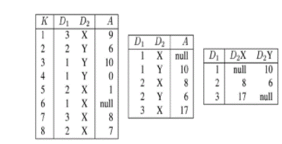
| Figure 1.shows an example. F is the base table. The result of vertical aggregation is stored in FV and that of horizontal
aggregation is stored in FH [11]. SQL query for FV is written as: |
| SELECT D1, D2, sum(A) |
| FROM F |
| GROUP BY D1, D2 |
| ORDER BY D1, D2; |
| As seen in fig. 1, sample data is given in input table. Vertical aggregation result is presented in (b). In fact the result
generated by SUM function of SQL is presented in (b). Horizontal aggregation results are presented in (c). .In FV, D2
consist of only two distinct values X and Y and is used to transpose the table. The aggregate operation is used in this is
sum (). The values within D1 are repeated, 1 appears 3 times, for row 3, 4 and, and for row 3 & 4 value of D2 is X & Y.
So D2X and D2Y are newly generated columns in FH. |
IV. QUERY EVALUATION METHODS |
| A new class of aggregations, i.e; horizontal aggregations have similar behaviour to SQL standard aggregations, but
which produce tables with a horizontal layout. HA (Horizontal Aggregation) can be evaluated by using three different
methods: |
| SPJ Method |
| CASE Method |
| PIVOT Method |
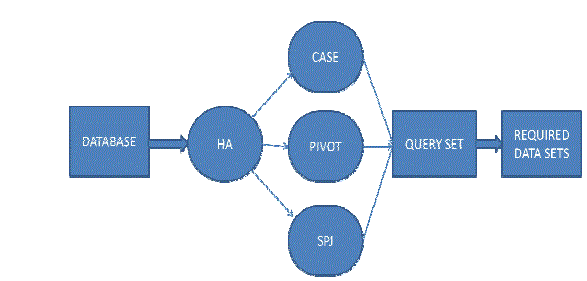
| Figure below shows the process flow for getting datasets in a horizontal layout using three different query evaluation
methods. |
| A. SPJ Method: |
| A. SPJ Method:
It is based on standard relational algebra operators (SPJ queries). The basic idea is to create one table with a vertical
aggregation for each result column, and then join all those tables to produce another table. It is necessary to introduce
an additional table F0 that will be outer joined with projected tables to get a complete result set. |
| INSERT INTO F0 |
| SELECT DISTINCT D1 |
| FROM F; |
| The optimized SPJ method code is follows: |
| INSERT INTO FH |
| SELECT F0.L1, F0.L2,....,F0.Lm, |
| F1.A, F2 .A,......,Fn .A |
| FROM F0 |
| LEFT OUTER JOIN F1 |
| ON F0. L1= F1. L1 and. . . and F0. Lm= F1. Lm |
| LEFT OUTER JOIN F2 |
| ON F0. L1= F2. L1 and. . . and F0. m= F2. Lm |
| . . . . |
| LEFT OUTER JOIN Fn |
| ON F0. L1= Fn. L1 and. . . and F0. Lm= Fn. Lm |
| Example: The SPJ code for getting FH as shown in fig.1 can be written as: |
| INSERT INTO F1 |
| SELECT D1, sum (A) AS A |
| FROM F |
| WHERE D2 = ‘X’ |
| GROUP BY D1; |
| INSERT INTO F2 |
| SELECT D1, sum (A) AS A |
| FROM F |
| WHERE D2 = ‘Y’ |
| GROUP BY D1; |
| INSERT INTO FH |
| SELECT F0.D1, F1.A AS D2_X, F2.A AS D2_Y |
| FROM F0 LEFT OUTER JOIN F1 on F0. D1 = F1. D1 |
| LEFT OUTER JOIN F2 on F0. D1 = F2. D1 |
| B. CASE Method: |
| It can be used in any statement or clause that allows a valid expression. The case statement returns a value selected
from a set of values based on Boolean expression. The Boolean expression for each case statement has a conjunction of
K equality comparisons. Query evaluation needs to combine the desired aggregation with “case” statement for each
distinct combination of values of R1;R2……..,Rk. The optimized case method code is as follows: |
| SELECT DISTINCT R1,…..,Rk |
| FROM Fv; |
| INSERT INTO FH |
| SELECT L1,L2,....,Lm |
| ,sum(CASE WHEN R1=v11 and . . . Rk=vk1 |
| THEN A ELSE null END) |
| .... |
| ,sum(CASE WHEN R1=v1n and . . . Rk=vkn |
| THEN A ELSE null END) |
| FROM Fv |
| GROUP BY L1,L2,. . .,Lm ; |
| Example: The code using CASE method for getting FH as shown in fig.1 can be written as: |
| INSERT INTO FH |
| SELECT |
| D1 |
| , SUM(CASE WHEN D2 = ‘X’ THEN A |
| ELSE null END) as D2_X |
| , SUM (CASE WHEN D2 = ‘Y’ THEN A |
| ELSE null END) as D2_Y |
| FROM F |
| GROUP BY D1; |
| C. PIVOT Method: |
| The pivot operator is a built-in operator which transforms row to columns. It internally needs to determine how many
columns are needed to store the transposed table and it can be combined with the GROUP BY clause. Since this
operator can perform transposition it can help in evaluating horizontal aggregation. The optimized PIVOT method SQL
is as follows: |
| SELECT DISTINCT R1 |
| FROM F; /*produces v1,………,vd*/ |
| SELECT |
| L1,L2,…,Lm |
| ,v1,v2,….,vd |
| INTO FH |
| FROM ( |
| SELECT L1,L2,…..,Lm, R1,A |
| FROM F) Ft |
| PIVOT( |
| V(A) FOR R1 in (v1,v2,…,vd) |
| ) AS P; |
| Example: The code using PIVOT method for getting FH as shown in fig.1 can be written as: |
| INSERT INTO FH |
| SELECT |
| D1 |
| , [X] as D2_X |
| , [Y] as D2_Y |
| FROM ( |
| SELECT D1, D2, A FROM F |
| ) as p |
| PIVOT ( |
| SUM (A) |
| FOR D2 IN ([X], [Y]) |
| ) as pvt; |
V. EXAMPLE OF GENERATED DATA SETS: SPJ AND CASE |
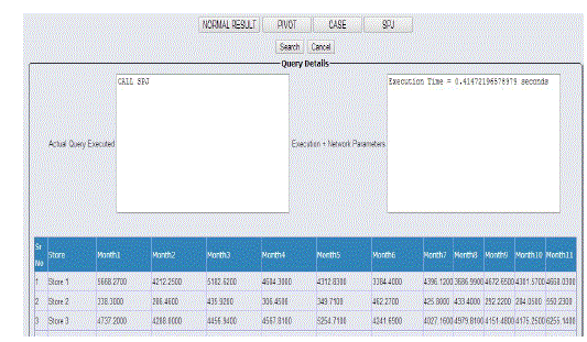
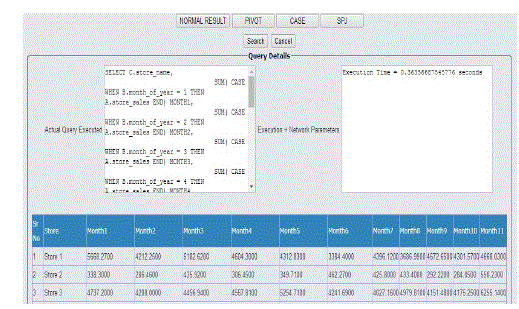
| We now show actual SQL code for our data sets which are shown in Fig. 3 & Fig. 4. This SQL code produces data sets
in a horizontal layout using SPJ and CASE methods.
The SPJ method code is as follows (computed from F): |
| /* SPJ method */ |
| BEGIN |
| SET @Query = 'SELECT C.store_name, '; |
| IF Duration = 'MONTHWISE' THEN |
| SET @Query = CONCAT(@QUERY, |
| 'TRUNCATE ((SUM( CASE WHEN B.month_of_year = 1 THEN ', Onvalue,' END)), 0) MONTH1, |
| TRUNCATE ((SUM( CASE WHEN B.month_of_year = 2 THEN ', Onvalue,' END)), 2) MONTH2, |
| TRUNCATE ((SUM( CASE WHEN B.month_of_year = 3 THEN ', Onvalue,' END)), 2) MONTH3, |
| TRUNCATE ((SUM( CASE WHEN B.month_of_year = 4 THEN ', Onvalue,' END)), 2) MONTH4, |
| TRUNCATE ((SUM( CASE WHEN B.month_of_year = 5 THEN ', Onvalue,' END)), 2) MONTH5, |
| TRUNCATE ((SUM( CASE WHEN B.month_of_year = 6 THEN ', Onvalue,' END)), 2) MONTH6, |
| TRUNCATE ((SUM( CASE WHEN B.month_of_year = 7 THEN ', Onvalue,' END)), 2) MONTH7, |
| TRUNCATE ((SUM( CASE WHEN B.month_of_year = 8 THEN ', Onvalue,' END)), 2) MONTH8, |
| TRUNCATE ((SUM( CASE WHEN B.month_of_year = 9 THEN ', Onvalue,' END)), 2) MONTH9, |
| TRUNCATE ((SUM( CASE WHEN B.month_of_year = 10 THEN ', Onvalue,' END)), 2) MONTH10, |
| TRUNCATE ((SUM( CASE WHEN B.month_of_year = 11 THEN ', Onvalue,' END)), 2) MONTH11') ; |
| END IF; |
| IF Duration = 'QUARTERWISE' THEN |
| SET @Query = CONCAT(@QUERY, |
| TRUNCATE ((SUM( CASE WHEN B.quarter = "Q1" THEN ', Onvalue,' END)), 0) QUARTER1, |
| TRUNCATE ((SUM( CASE WHEN B.quarter = "Q2" THEN ', Onvalue,' END)), 2) QUARTER2, |
| TRUNCATE ((SUM( CASE WHEN B.quarter = "Q3" THEN ', Onvalue,' END)), 2) QUARTER3, |
| TRUNCATE ((SUM( CASE WHEN B.quarter = "Q4" THEN ', Onvalue,' END)), 2) QUARTER4') ; |
| END IF; |
| IF Duration = 'YEARWISE' THEN |
| SET @Query = CONCAT(@QUERY, ' TRUNCATE((SUM( ',Onvalue,')), 2) YEAR1') ; |
| END IF; |
| SET @Query = CONCAT(@QUERY, ' FROM sales_fact_1998 A |
| LEFT JOIN time_by_day B ON B.time_id = A.time_id |
| LEFT JOIN store C ON C.store_id = A.store_id |
| GROUP BY A.store_id'); |
| PREPARE STMT FROM @Query; |
| EXECUTE STMT; |
| END |
| The CASE method code is as follows (computed from F): |
| /* CASE method */ |
| SELECT C.store_name, |
| SUM( CASE WHEN B.month_of_year = 1 THEN A.store_sales END) MONTH1, |
| SUM( CASE WHEN B.month_of_year = 2 THEN A.store_sales END) MONTH2, |
| SUM( CASE WHEN B.month_of_year = 3 THEN A.store_sales END) MONTH3, |
| SUM( CASE WHEN B.month_of_year = 4 THEN A.store_sales END) MONTH4, |
| SUM( CASE WHEN B.month_of_year = 5 THEN A.store_sales END) MONTH5, |
| SUM( CASE WHEN B.month_of_year = 6 THEN A.store_sales END) MONTH6, |
| SUM( CASE WHEN B.month_of_year = 7 THEN A.store_sales END) MONTH7, |
| SUM( CASE WHEN B.month_of_year = 8 THEN A.store_sales END) MONTH8, |
| SUM( CASE WHEN B.month_of_year = 9 THEN A.store_sales END) MONTH9, |
| SUM( CASE WHEN B.month_of_year = 10 THEN A.store_sales END) MONTH10, |
| SUM( CASE WHEN B.month_of_year = 11 THEN A.store_sales END) MONTH11 |
| FROM sales_fact_1998 A |
| LEFT JOIN time_by_day B ON B.time_id = A.time_id |
| LEFT JOIN store C ON C.store_id = A.store_id |
| GROUP BY A.store_id. |
VI. EXPERIMENTAL EVALUATION AND ANALYSIS |
| The prototype is web based application which is built using the environment containing a PC with 4 GB RAM, core i3
processor running Windows 8 operating system. The application is built using XAMPP package, where PHP is used as
coding language and MySQL server is used as backend. MySQL server does not support the PIVOT keyword. So we
will see the aggregated datasets using SPJ and CASE method only. |
| As seen in fig. 3, SPJ operation’s results are presented in horizontal layout. This kind of data can be used further for
data mining operations. In this figure we can see that the SPJ procedure is called to get the datasets, that procedure has
been created and stored in the database once it is executed. In this way, time can be saved. Likewise number of
procedures can be stored in a query set and unavailable queries can also be created dynamically. |
| As seen in fig. 4, CASE operation’s results are presented in horizontal layout. This kind of data can be used further for
data mining operations. In this case, the procedure is not created for explanation purpose. As PIVOT keyword is not
available in MySQL, we were unable to get the data sets using PIVOT method. |
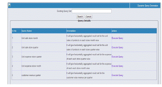
| Fig.5 shows the query set, which consists of some procedures, so whenever user wants to use any one of those
procedures, just click on execute query and the resulting datasets will be displayed on the screen. |
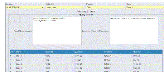
| If the procedure is not available for a required query in query set then the user can go for dynamic query generation. For
dynamic query generation user has to select some parameters and need to click on build query, the data sets will be
showed for respective query in new tab. If user wants to save dynamically generated query then that option is also
provided. User can save the query by giving any name and it will be automatically saved in the available query set. |
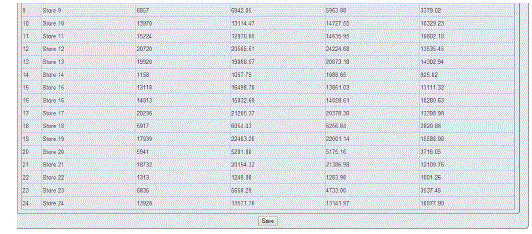
| Above figure shows the screen for generating dynamic queries. Dynamic queries are those which are not available in the
available query set but just by passing the parameters in the fields from required query, user can get the result of query
within no time and that query can be saved by using SAVE option provided in the same form which has been shown in
the fig. 7. |
| By using this ‘save’ option, user can save the query not data set so whenever the query will be executed in future, user
will always get the refresh data sets. These queries are stored in the available query set. |
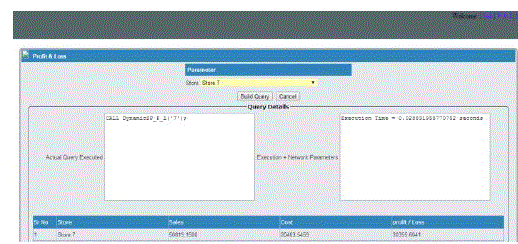
| This screen shows one Profit and Loss (P&L) tab to calculate the profit or loss for individual stores. This is one of the
applications mentioned above to get the data sets for analysing purpose. In the way we can use our HA methods to
simplify the analysis of data sets using our created query sets which makes easy to get the data sets within no time. |
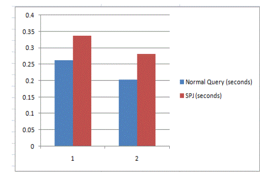
| Analysis: In this project we have distinguished the HA methods from vertical aggregation method. Though the time
taken by HA methods is more as compared to the vertical aggregations but the resulting data sets produced by using
HA methods is more feasible and easy to analyse. Hence, we can summarize the topic by showing the graph in fig.9,
which shows the accuracy and time complexity of HA as well as vertical aggregations. |
VII. CONCLUSION AND FUTURE WORK |
| A new class of aggregate functions in SQL called horizontal aggregation is used that helps for making datasets for the
data mining projects. These functions are used for creating query sets which gives the resultant data sets in a horizontal
layout, because most of the data mining algorithms require datasets in horizontal layout. Mainly, the existing SQL
aggregations return results in one column per aggregated group. But in horizontal aggregation, it returns a set of numbers
instead of a single number for each group. Three query evaluation methods are proposed. |
| The first method focuses on the relational operators in SQL. The second method focuses on the SQL case construct. The
third method focuses on the PIVOT built-in operator in a commercial DBMS. By analysing, it is observed that the HA
methods are more accurate and feasible as compared to the vertical aggregation method. Horizontal aggregation
produces tables with fewer rows but with more columns. So the traditional query optimization techniques are
inappropriate for the new class of aggregations. So the next plan is to develop the most appropriate query optimization
technique for the horizontal aggregation to achieve better results. Then we can also develop more complete I/O cost
models. |
Figures at a glance |
 |
 |
 |
 |
 |
| Figure 1 |
Figure 2 |
Figure 3 |
Figure 4 |
Figure 5 |
 |
 |
 |
 |
| Figure 6 |
Figure 7 |
Figure 8 |
Figure 9 |
|
| |
References |
- C. Ordonez, “Data Set Preprocessing and Transformation in a Database System,” Intelligent Data Analysis, vol. 15, no. 4, pp. 613- 631, 2011.
- C. Ordonez and S. Pitchaimalai, “Bayesian Classifiers Programmed in SQL,” IEEE Trans. Knowledge and Data Eng., vol. 22, no. 1, pp. 139-144, Jan. 2010.
- C. Ordonez, “Statistical Model Computation with UDFs,” IEEE Trans. Knowledge and Data Eng., vol. 22, no. 12, pp. 1752-1765, Dec. 2010.
- Han and M. Kamber, Data Mining: Concepts and Techniques, first ed. Morgan Kaufmann, 2001.
- S. Sarawagi, S. Thomas, and R. Agrawal, “Integrating Association Rule Mining with Relational Database Systems: Alternatives andImplications,” Proc. ACM SIGMOD Int’l Conf. Management of Data (SIGMOD ’98), pp. 343-354, 1998.
- H. Wang, C. Zaniolo, and C.R. Luo, “ATLAS: A Small But Complete SQL Extension for Data Mining and Data Streams,” Proc. 29th Int’l Conf. Very Large Data Bases (VLDB ’03), pp. 1113- 1116, 2003.
- Witkowski, S. Bellamkonda, T. Bozkaya, G. Dorman, N. Folkert, A. Gupta, L. Sheng, and S. Subramanian, “Spreadsheets in RDBMS forOLAP,” Proc. ACM SIGMOD Int’l Conf. Management of Data (SIGMOD ’03), pp. 52-63, 2003.
- Ordonez, “Vertical and Horizontal Percentage Aggregations,” Proc. ACM SIGMOD Int’l Conf. Management of Data (SIGMOD ’04), pp. 866-871, 2004.
- Ordonez, “Integrating K-Means Clustering with a Relational DBMS Using SQL,” IEEE Trans. Knowledge and Data Eng., vol. 18, no. 2, pp.188-201, Feb. 2006.
- J. Clear, D. Dunn, B. Harvey, M.L. Heytens, and P. Lohman, “Non- Stop SQL/MX Primitives for Knowledge Discovery,” Proc. ACMSIGKDD Fifth Int’l Conf. Knowledge Discovery and Data Mining (KDD ’99), pp. 425-429, 1999.
- Carlos Ordonez and Zhibo Chen, (2012), “Horizontal Aggregations in SQL to Prepare Data Sets for Data Mining Analysis”, IEEE Trans. Knowledge and Data Eng., Vol. 24, No. 4., April 2012.
|