ISSN ONLINE(2319-8753)PRINT(2347-6710)
ISSN ONLINE(2319-8753)PRINT(2347-6710)
Nilesh Pohokar 1, Lalit Bhuyar2
|
| Related article at Pubmed, Scholar Google |
Visit for more related articles at International Journal of Innovative Research in Science, Engineering and Technology
To select the optimum parameters it is necessary to determine them at first for the given machining situation. There are several techniques available to determine the optimum values of these parameters, in this paper machining parameters, cutting speed, feed, depth of cut, and one geometric parameter rake angle are considered for optimization. The neural networks were developed for predicting the results theoretically. To validate the results experimentally trials are then carried out a CNC milling using HSS tool by continuous running condition under dry run on the AISI 1040 MS plate of 140 X 120 X 10 mm workpiece. The predicted results match 90 % including the residuals. Thus proves the neural network is used for optimization of geometric and machining parameters.
Keywords |
| Geometric parameter, Machining parameters ANN, CNC milling, Tool life |
INTRODUCTION |
| The main objective of this paper is to optimize the geometric and machining parameters of parallel shank end mill tool. The selection of machine, workpiece and machine tools are very important for the optimization of machining and geometric parameters. These parameters are directly caused the tool wear and life of the tool. There are several methods of optimization, this methods gives the optimization procedure which is utilized for improvements in tool life. A scientific approach to plan the experiments is a necessity for efficient conduct of experiments. By the statistical design of experiments the process of planning the experiment is carried out, so that appropriate data will be collected and analysed by statistical methods resulting in valid and objective conclusions. When the problem involves data that are subjected to experimental error, statistical methodology is the only objective approach to analysis. Thus, there are two aspects of an experimental problem: the design of the experiments and the statistical analysis of the data. These two points are closely related since the method of analysis depends directly on the design of experiments employed. The advantages of design of experiments are as follows: • Numbers of trials is significantly reduced. • Important decision variables which control and improve the performance of the tool can be identified. • Optimal setting of the parameters can be found out. • Qualitative estimation of parameters can be made. • Experimental error can be estimated. • Inference regarding the effect of parameters on the characteristics of the process can be made. In this paper before going for all this optimization procedure first the industrial data related to tool failure, tool wear rate life of the tool, tool changing time before starting a new batch is collected. Some trial experiments are perform by continuous running under dry run condition on non optimize tool until the desired flank wear and face wear occurs, for calculating the tool wear rate and tool life. |
| 1. Selection of Machine: The selection of machine is important because the optimization procedure is considered for machining parameters. First the survey is conducted for the same machine specification utilize for different operation. In this work considering those machining parameters is same for other machines. It is better to utilize a machine which is experimentally ideal and have the same specification with respect to machining parameters. In CNC milling machine same procedure is applied for optimization to find out the greater tool life by selecting the same machining and geometric parameters at different operation. 2. Study of Tool wear and Tool wear criteria Flank Wear: It is caused by the friction between the newly machined work piece surface and the tool flank face. It is responsible for a poor surface finish, a decrease in the dimension accuracy of the tool and an increase in cutting force, temperature and vibration. |
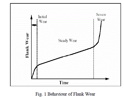 |
| Hence the width of the flank wear land “VB” is usually taken as a measure of the amount of wear and a threshold value of the width is defined as tool reshape criterion. Fig. 1 shows a variation of flank wear rate with cutting time, showing the initial wear, steady wear, and severe wear periods. The maximum acceptable flank wears of 0.30 mm as recommended by machine tool hand book by central machine tool institute. Face Wear: It is the wear in which contact with chips erodes the rake face. This is somewhat normal for tool wear, and does not seriously degrade the use of a tool until it becomes serious enough to cause a cutting edge failure can be caused by spindle speed that is too low or a feed rate that is too high. In milling it may occur where the tool temperature is highest. Face wear occurs approximately at a height equating the cutting depth of the material. In our work cutting depth is 0.25 mm as recommended by machine tool hand book by central machine tool institute. Prediction of Tool Wear: Prediction of tool wear is complex because of the complexity of machining system. Tool wear in cutting process is produced by the contact and relative sliding between the cutting tool and the work piece and between the cutting tool and under the extreme conditions of cutting area; temperature at the cutting edge can exceed 500°C and pressure is greater than 15 N/mm2. The wear of the tool is dependent on elements as- whole machining system comprising work piece, tool, interface and machine tool. |
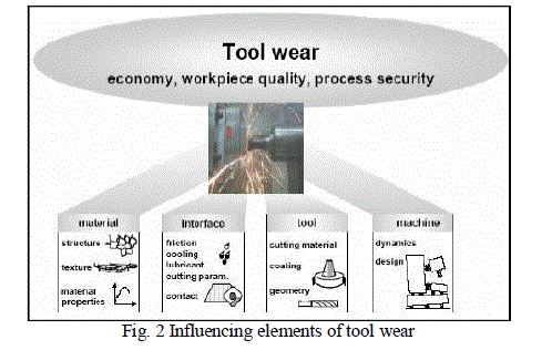 |
| Work Piece: It includes the work piece material and its physical properties (mechanical and thermal properties, microstructure, hardness, etc), which determine energy for the applied cutting conditions. Tool: Tool material, tool coatings and tool geometric design (edge preparation, rake angle, etc) need to be appropriately chosen for different operations (roughing, semi roughing, or finishing). The optimal performance of a cutting tool requires a right combination of the above tool parameters and cutting conditions (cutting speed, feed rate, depth of cut). Interface: It involves the interface conditions. In 80% of the industrial cutting applications, coolants are used to decrease cutting temperatures and likely reduce tool wear. Increasingly new technologies, such as the minimum liquid lubrication, have been developed to reduce the cost of coolant that makes up to 16% of the total machining costs. Dynamic: The dynamic characteristic of the machine tool, affected by the machine tool structure and all the components taking part in the cutting process, plays an important role for a successful cutting. Instable cutting processes with large vibrations (chatters) result in a fluctuating overload on the cutting tool and often lead to the premature failure of the cutting edge by tool chipping and excessive tool wear. The problem of tool wear monitoring in machining operation has been active area of research. This is because tool change strategies, product quality, tooling costs, and productivity are all influenced by tool wear. Reduction in production cost and increase in productivity can be realized by making the most use of a tools life and therefore increasing the time between tool changes. 3. Effects of Tool Wear On Technological Performance • Decrease the dimension accuracy • Increase the surface roughness • Increase the cutting force • Increase the temperature • Likely cause vibration • Lower the production efficiency, component quality • Increase the cost. 4. Tool Failure Modes and Tool Life A tool can be considered to have failed when it has worn sufficiently where the dimensional tolerance and surface finish are impaired or when catastrophic failure occurred. Tool failure modes have been used to establish tool life criteria. Armarego et al. [08] have listed tool life criterion as follows: • Chipping or fine cracks developing at the cutting edge wear land size on the clearance surface. • Crater depth or other parameter of the crater on the rake face. • Volume or weight of material worn off the tool. Total destruction of the cutting tool. These criteria by itself or in combination could be used to determine tool failure. Tool failure is also characterized by its flank wear, crater wear, cracking and chipping of the tool. |
II. LITERATURE REVIEW |
| M. Nalbanta, H. kkayab [20] explains the experimental investigation of the effects of uncoated, PVD-and CVDcoated cemented carbide insert sand cutting parameters on surface roughness in CNC turning and its prediction using artificial neural networks The machining of AISI1030 steel (i.e. orthogonal cutting) uncoated, PVD and CVD-coated cemented carbide insert with different feed rates of 0.25, 0.30, 0.35, 0.40 and 0.45 mm/rev with the cutting speeds of 100, 200 and 300 m/min by keeping depth of cuts constant (i.e.2mm), without using cooling liquids has been accomplished. The surface roughness effects of coating method, coating material, cutting speed and feed rate on the work piece have been investigated. Among the cutting tools with 200 mm/min cutting speed and 0.25mm/rev feed rate the TiN coated with PVD method has provided 2.16 mm, TiAlN coated with PVD method has provided 2.3 mm, AlTiN coated with PVD method has provided 2.46 mm surface roughness values, respectively. While the uncoated cutting tool with the cutting speed of 100m/min and 0.25mm/rev feed rate has yielded the surface roughness value of 2.45 mm. After wards, these experimental studies were executing artificial neural net works (ANN). The training and test data of the ANNs have been prepared using experimental patterns for the surface roughness. In the input layer of the ANNs, the coating tools, feed rate (f) and cutting speed (V) values are used while at the output layer the surface roughness values are used. They are used to train and test multilayered, hierarchically connected and directed networks with varying numbers of the hidden layers using back-propagation scaled conjugate gradient (SCG) and Leven berg–Marquardt(LM) algorithms with the logistic sigmoid transfer function. The experimental values and ANN predictions are compared by statistical error analyzing methods. It is shown that the SCG model with nine neurons in the hidden layer has produced absolute fraction of variance (R2) values about 0.99985for the training data, and 0.99983 for the test data; root mean square error(RMSE) values are smaller than 0.00265; and mean error percentage (MEP) are about 1.13458 and 1.88698 for the training and test data, respectively. Karpat & Ozel [19] introduce a procedure to formulate and solve optimization problems for multiple and conflicting objectives that may exist in turning processes. Advanced turning processes, such as hard turning, demand the use of advanced tools with specially prepared cutting edges. It is also evident from a large number of experimental works that the tool geometry and selected machining parameters have complex relations with the tool life and the roughness and integrity of the finished surfaces. The non-linear relations between the machining parameters including tool geometry and the performance measure of interest can be obtained by neural networks using experimental data. The neural network models can be used in defining objective functions. In this study, dynamic neighborhood particle swarm optimization (DN-PSO) methodology is used to handle multi-objective optimization problems existing in turning process planning. The objective is to obtain a group of optimal process parameters for each of three different case studies presented in this work. The case studies considered in this study are: minimizing surface roughness values and maximizing the productivity, maximizing tool life and material removal rate, and minimizing machining induced stresses on the surface and minimizing surface roughness. The optimum cutting conditions for each case study can be selected from calculated Pareto-optimal fronts by the user according to production planning requirements. The results indicate that the proposed methodology which makes use of dynamic-neighborhood particle swarm approach for solving the multi objective optimization problems with conflicting objectives is both effective and efficient, and can be utilized in solving complex turning optimization problems and adds intelligence in production planning process. The critical review of the literature also suggested that inadequate work is done on optimization of geometric parameters w. r. t. tool life estimations. Many researchers are engaged in the study the correlation between the surface roughness’s, shape change, feed rate control and optimize cutting speed in terms of the tool life, tool path generation algorithm of the milling operations. |
| A neuron is the basic element of neural networks, and its shape and size may vary depending on its duties. Analyzing a neuron in terms of its activities is important, since understanding the way it works also help us to construct the ANNs. An ANN may be seen as a black box, which contains hierarchical sets of neurons (i.e. processing elements) producing outputs for certain inputs. Each processing element consists of data collection, processing the data and sending the results to the relevant consequent element. Each processing element consists of data collection, processing the data and sending the results to the relevant consequent element. The whole process may be viewed in terms of the inputs, weights, the summation function and the activation function |
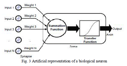 |
| 1. The inputs are the activity of collecting data from the relevant sources. 2. The weights control the effects of the inputs on the neuron. In other word an ANN saves its information over its links and each link has a weight. These weights are constantly varied while trying to optimize the relation between the inputs and outputs. 3. Summation function calculates of the net input readings from the processing elements. 4. Transfer (activation) function determines the output of the neuron by accepting the net input provided by the summation function. There are several transfer functions like summation function. Depending on the nature of the problem the determination of transfer and summation function is made. A transfer function generally consists of algebraic equations of linear or nonlinear form [9]. The use of a nonlinear transfer function makes a network capable of storing nonlinear relationships between the input and the output. A commonly used function is sigmoid function because it is self-limiting and has a simple derivative. An advantage of this function is that the output cannot grow infinitely large or small [10]. 5. Outputs accept the results of the transfer function and present them either to the relevant processing element or to the outside of the network. The functioning of ANNs depends on their physical structure. An ANN may be regarded as a directed graph containing a summation function, a transfer function, its structure and the learning rule used in it. The processing elements have links between them forming a layer of networks. A neural network usually consists of an input layer, a number of hidden layers and an output layer. 1. Determination of data and the network model The training and test data have been prepared using experimental patterns. In this work, the 13 patterns have been randomly selected and used as the test data. Cutting speed, Depth of cut, feed rate, rake angle have been used as input layer, while the tool life was used as output layer of the ANNs. In the ANN model logistic transfer function has been used and expressed as |
 |
| Where, NETi weighted sum of the input and output values are normalized between 0 and 1. Wij weights of the connections between ith and jth processing elements wbi weights of the biases between layers 2 The training of the network Generally, there are three different learning strategies. First, the trainer may tell the network what it should learn (Supervised Learning), second, the trainer may indicate whether or not the output is correct without telling what the network should learn (Reinforcement Learning) and finally, the network learns without any intervention of the trainer (Unsupervised Learning). The learning set consists of the inputs and the outputs used in training the network. The required outputs take place in this set in the case of supervised learning, while in other cases, they are not found in it [19]. In our work we have used supervised learning approach. Since the number of neurons found in the input and output layers are known, the best performance of the network with the number of hidden layers is determined. |
 |
| The neural network is developed under Decision tool Suite 6.2 trial version software used. In the first step of the training, a determination of the learning algorithms is made. The number of hidden layers and the number of neurons for each hidden layer are determined. Then, the number of iterations is entered, and the training starts. The training continues either to the end of the iterations or reaching the target level of errors |
IV. METHODOLOGY |
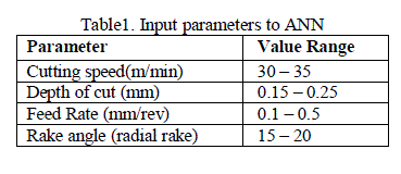
| 1. Input to ANN Due to geometry of parallel shank end mill tool parameter and machining parameters the cutting process is complex and involves a large number of interdependent variables that define the machining condition. In this work, four key input variables are considered shown in table on the other hand, helix angle, diameter, clearance angle, and number of flutes are kept constant. |
 |
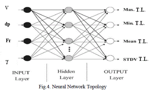
| Thus, the input vector to the ANN that represents the variable cutting parameters can be written as follows: Input = [V, Fr, dp, γ] 2. Output from ANN The maximum, minimum, mean and standard deviation values of the tool life are used to represent the instantaneous cutting force; thus, resulting in the following output (or target) vector. Output (or target) = [max (T.L.), min (T.L.), mean (T.L.), STDV(T.L.)] |
 |
| Where, Max(T.L.) stands for maximum of T.L. Min (T.L.) stands for minimum of T.L. Mean (T.L.) stands for mean of T.L STDV (T.L.) stands for standard deviation of T.L. Using the above input and output vectors, the resulting topology of the ANN becomes as shown in fig. 4. 3. Steps of optimization for Geometric and Machining Parameters |
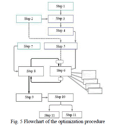 |
| The Fig.5 shows the algorithm flowchart of the optimization procedure Step 1: Enter the input data: The following input data must be entered into the model Cutting speed, Feed Rate, Depth of Cut, Rake Angle Step 2: Generation of random cutting conditions. The extent of conditions can be changed optionally. Step 3: Calculation methodology for tool life Step 4: Preparation of data for training and testing of ANN. Uniting of cutting conditions and other calculated values into a data matrix. Normalization of the data in the matrix follows. All data must have their values between 0–1. There is Breakdown of the data matrix into the input and output vector. Distribution of the input/output vector into the two sets for training and testing. |
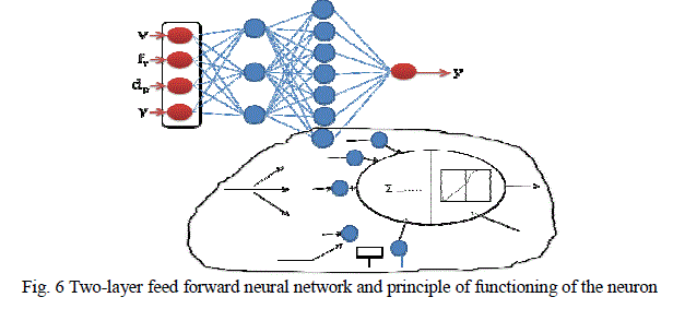
| Step 5: Use of ANN. The purpose of the neural network is to predict the Tool Life (T.L.) in case of randomly selected cutting conditions. Step 6: Selection of the type and architecture of the ANN and searching for optimum training parameters. Step 7: Procedure of training of the ANN by using the training set. Step 8: Testing of trained ANN. If testing is successful and the error of prediction is within the permissible limits, the empirical model is finished and ready for use. In case the testing is not successful, the training procedure must be repeated with another larger set of training data or the training parameters must be changed. Step 9 : Post processing of data. Step 10: Process of optimization: For the optimization process Decision tool Suite 6.2 trial version software used. The cutting conditions where the tool life (T. L.) has the maximum are the optimum cutting conditions. The extreme of tool life (T.L.) with consideration of the limitation equations is searched for. Since the tool life (T.L.) is expressed with ANN, it means that the extreme of the neural network is searched for. The procedure is theoretically completely identical with searching for the extreme of the tool life with several variables. The area in which the extreme is searched for is defined with limitation equations. The procedure does not find the minimum located outside the defined area. The procedure ensures also fine tuning (searching) of the global minimum when the process stops in the local minimum. Step 11: Graphic representation of results and optimization statistic. The described procedure is fully automated although also interactive method. 4. Architecture & Adaptation for optimization The two-layer feed forward neural network has proved to be an excellent universal approximation of non-linear functions [20]. If it is capable of approximating any nonlinear function, than it is possible to represent with it any manufacturer’s implicit multi attribute function. The ANN needs four input neurons for three machining parameters and one geometric parameter. If the values are not at the same scale, all data must be normalized. The output from the neural network is a real value tool life (T.L.), therefore only one output neuron is necessary given in fig. 6 |
 |
| 5. Development of neural network to Decision tool Suite 6.2 trial version software : The Decision Tools Suite is an integrated set of programs for risk analysis and decision making under uncertainty that runs in Microsoft Excel. The Decision Tools Suite includes for neural tools for predictive neural networks, and optimizer for optimization. In this work the geometric and machining parameters are optimized to achieve better results. |
V. EXPERIMENTAL SETUP |
| One of the main objectives of this experiment is to increase the tool life to reduce the flank wear by optimizing the cutting and geometric parameter. Flank wear is measured on tools makers’ microscope. It is very difficult to consider all factors while calculating the tool life. So for this work, the tool life is dependent on feed, depth of cut, speed, and rake angle. (Considering three cutting parameter and one geometric parameter) The development of an equation for tool life, rake angle, depth of cut, feed rate, cutting speed into an economic model for the prediction of speed and feed values; and hence Estimating the optimum tool life. |
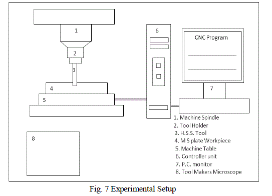
| Due to the limitation of infrastructure facilities for making the desired angles, decision are made only one geometric parameter tool radial rake angle is modified. In this work only one geometric parameter is considered and other parameters such as helix angle, end cutting edge concavity angle, axial and radial relief angle are kept constant. This radial rake angle is supplied by the supplier as per the requirement and tested in the laboratory with the help of bevel protector and marked. Also the three machining parameters spindle speed, feed and depth of cut and other kept constant. The CNC machine is utilized to make control and accurate measurement of these parameters on the screen of display monitor. All the ranges of value of selected parameters are taken as per hand book recommendation selected values. Proper experimental plan is necessary to achieve good results in conducting research. The scheme of carrying out experiments was selected and the experiments were conducted to investigate the effect of geometric and machining parameters on the output parameters such as tool wear and tool life calculation. The factors and their levels considered in this study whereby conduct with four factor with three level experiments. The experimental studies were performed on Sinewave VMM-T-200 vertical machining machine using MS plate (AISI1040) as a work piece and HSS parallel shank end mill tool of M2/14/J/4F grade as a tool. Fig.7 indicates the diagrammatic representation of the experimental set up. |
 |
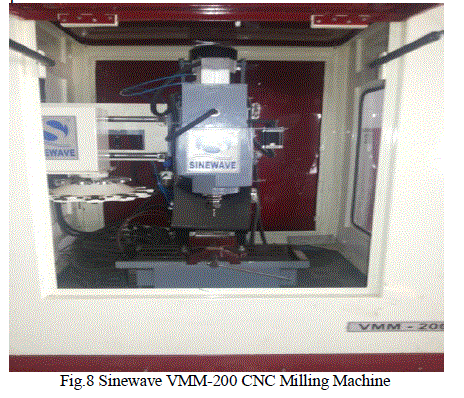
| The readings of the experimentation in term of tool wear are considered as per the prediction given by optimization procedure. In experimental work the 140 minute time is set for all the trials and then machine will be stopped to record the following readings. • Flank wear (5 readings per experiment) • Face wear (5 readings per experiment) • Weight of tool (5 readings per experiment) The flank wear and face wear are measured by tool maker’s microscope and the weight before and after the trial measured using precision balance machine. 1. CNC Vertical Milling Machine The experiments were carried out on 3-axis on Sinewave VMM-T-200 vertical machining machine as shown in Fig.8 This CNC Machine is a quality product of sinewave Engineering Pvt. Ltd., Pune capable of performing multiple operations with accuracy of 0.01 mm, quality and productivity. BMV45/T20/TC20/TC24 is a CNC Vertical machining Center consisting of main spindle, automatic tool changer, coolant system and Pneumatic system. It is designed for metal cutting, as a machine tool and can be used for machining materials like steel cast iron, aluminum, bronze & nonmetallic materials like acrylic. Components of VMC Machine are Machine body, CNC system, Electrical system, Pneumatic system, Coolant system Guards & Tool magazine (T20/TC24). The tests were carried out under dry condition with total of 9 experiments and another 3 experiment for the confirmation test. Total 35 holes were drilled by each drill in a predefined manner on each plate. A CNC part programs was prepared & executed for drilling operation. Experimentation are conducted on CNC Milling machine on the AISI 1040 MS plate work piece using 14MM parallel shank end mill tool for a rough milling operation under dry running continuous running condition for a period of 140 minute. During the experimentation the tool is unloaded 5 times at an interval of after performing the drilling operation of 7 holes. To check the flank wear, face wear and weight loss of tool. During loading and unloading the stop watch is use to note the start and stop time. |
 |
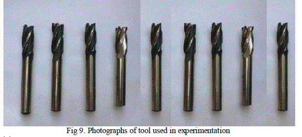
| 2. H.S.S. Tool Fig.9 shows a High speed steel (HSS), is a material usually used in the manufacture of machine tool bits and other cutters. It is often used in power saw blades and drill bits. It is superior to the older high carbon steel tools used extensively through the 1940s in that it can with stand higher temperatures without losing its temper (hardness). This property allows HSS to cut faster than high carbon steel, hence the name high speed steel. They are used widely of cutting operations that required complex shapes, example drilling, reamers, taps and gear cutters. Tungsten is the major alloying element but it is also combined with molybdenum, vanadium and cobalt in varying amounts. High Speed Steel cutting tools are available in many different tool geometries and material grades. While the choice of tool geometry varied with the type of cutting operation and the dimensions of the tool holder, the grade of the HSS tools used for experimentation were the same. There are two basic types of high speed steel, molybdenum (M series) and tungsten (T series). Generally, the M series has higher abrasion resistance than the T series due to M series undergoes less distortion during heat treating and is less expensive. Consequently, 98% of all high speed steel made of M-series steels. In order to improve the performance of high speed steel. This particular grade M2 was chosen for the experiments as it is most widely used in the industries because of its superior performance characteristics like good red-hardness and retains its cutting edge longer than other general purpose high speed steels. The chemical composition of this grade of tools (drills), as provided by the manufacturer, is as follows |
 |
 |
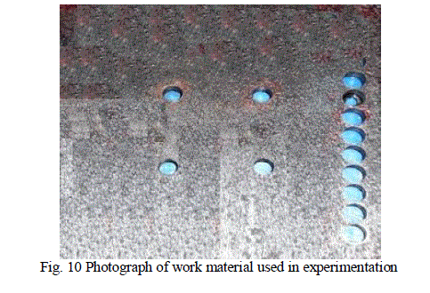
| 3. Work Material The work material used for the experimentation is a M.S. plate (Fig. 10) (AISI1040 steel) of 10 mm thickness. This main plate was cut in to number of square plates of size 140 X 120 X 10 mm. The chemical composition of this MS plate (AISI1040 steel) is as under |
 |
 |
VI. RESULTS AND DISCUSSIONS |
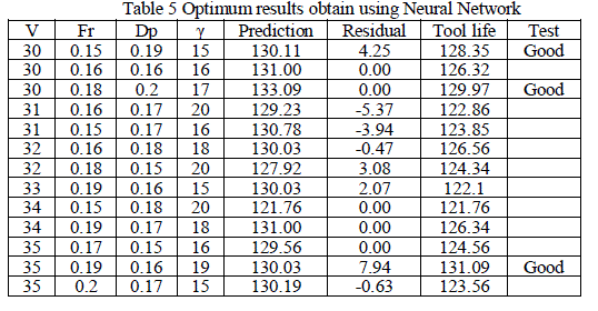
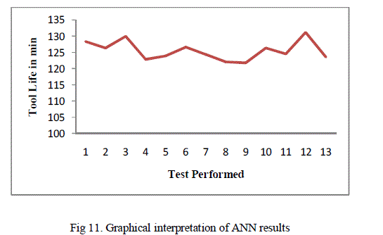
| 1. Neural Network Results ; As per results obtained by neural network the value of parameter where there is a greater tool life is consider for the test. So as per the prediction given the training and test are conducted on only the parameters which has greater tool life. The Table 4 shows the results and remarks of the test are conducted on the neural network. The results are calculated in the decision tools suite 6.2 trial version software is an integrated set of neural tool used in optimization run on Microsoft excel. |
 |
 |
 |
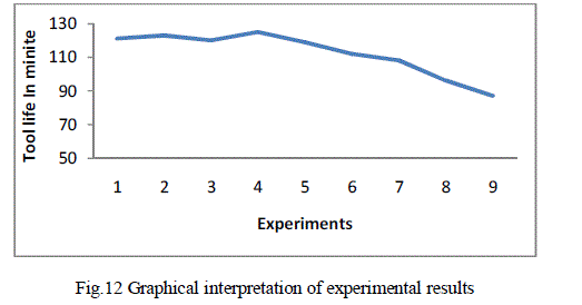
| 2. Experimentation Results Following are the experimental results obtain for the tool life which is directly observed form the experimentation shown in table 6. |
 |
 |
VII. CONCLUSION |
| The geometric and machining parameters are studied in order to optimize tool life to the greater extent. As per the handbook recommendation the parameters cause the tool wear which is directly proportional to tool life is studied and modified for better results. By understanding the concepts of establishing the values of geometric and machining parameters, the suitable optimization procedures for a wide variety of problem in the area of design and manufacturing was develop and implemented. The optimized values of geometric and machining parameters directly used in the manufacturing industry. The tool life obtains theoretically and experimentally when compared the 90% matching was found out because of residuals that can again be control and again optimized up to 95 %. This set a correct optimization procedure for optimizing the parameters. |
References |
|