ISSN ONLINE(2319-8753)PRINT(2347-6710)
ISSN ONLINE(2319-8753)PRINT(2347-6710)
Pruthviraj U1, Subhash C Yaragal2, M K Nagaraj3
|
| Related article at Pubmed, Scholar Google |
Visit for more related articles at International Journal of Innovative Research in Science, Engineering and Technology
A turbulent two dimensional flow behind perforated plate is numerically simulated and compared with the results of wind tunnel experiments from literature [1]. Realizable k-ε of the Fluent software is tested for the normal plates of porosities 0%, 10%, 20%, 30%, 40% and 50%, using which mean velocity, surface mean pressure and reattachment lengths were predicted inorder to study the fluid interaction and the size and shape of the bubble. Realizable k-ε turbulent model, which is an eddy-viscosity turbulence model, performed reasonably well for the thin perforated plate under study. For perforation greater than 30%, the simulation showed that the bubble is completely swept out as proved by the experiment.
Keywords |
| Realizable k-ε, perforated plate, turbulence modelling, reattachment length. |
INTRODUCTION |
| Concept of separation and reattaching flows are encountered in diverse fields ranging from aeronautics to hydraulics. During flow separation, the speed of the boundary layer relative to the solid body tends to zero and the fluid flow past the body gets detached from the surface; forming vortices. The potential of Computational Fluid Dynamics (CFD) has proved itself to be the powerful tool to solve problems involving fluid flows using numerical methods and algorithms. In the present study, numerical modeling for 2D flow field behind perforated plates on a flat surface has been done through CFD and verified with results available in literature. Study becomes relevant as the concept of fluid flow through perforated plates is one of the classic cases of fluid mechanics which has its importance in wide range of applications including designing aircraft, sediment transport, design of windbreaks for crop protection etc. The turbulence modelling is the key issue in numerical simulation. There have been several studies in literature to choose the appropriate turbulence model which can predict the experimental data with close proximity. The work of Packwood [2] compares the results of wind tunnel tests and CFD modelling for downstream of a two-dimensional porous fence in a thick boundary layer for porosities of 0%, 23% and 50%. Modified k-ε and full Reynolds stress models were the two turbulence models which were considered for the study. The k-ε model was adopted to incorporate a preferential dissipation modification (PDM). The „k-ε+ PDMâÃâ¬ÃŸ model was found to give a slightly better representation of the flow than the Reynolds stress (RS) model. Alhajraf [3] used computational fluid dynamics for two and three-dimensional simulation of wind-blown particles such as sand, soil or snow by using homogenous two-phase flow theory, where the flow field is predicted by solving Navier–Stokes equations for transient and incompressible viscous flow. Suitability of Computational Fluid Dynamics (CFD) with regard to windbreak aerodynamics was investigated by Bourdin et al. [4]. During the study, standard k–ïÃÂÃÂ¥ model, renormalization-group (RNG) k–ïÃÂÃÂ¥ model, realizable k–ïÃÂÃÂ¥ model were tested. On a fine grid, FluentâÃâ¬ÃŸs “realizable k–ïÃÂÃÂ¥ closure” yielded results that were in qualitative agreement with the observed mean winds. Yeh et al. [5] investigated the sheltering performance of porous windbreaks under various wind directions using 3D full scale storage yard model. RNG k -ïÃÂÃÂ¥ turbulence was used to study efficacy of rectangular wind fence, octagonal wind fence, octagonal wind fence with additional mid-fences in perpendicular and parallel directions etc. The simulation results revealed that the traditional rectangular wind fence configuration protects stock piles from the erosive effects of wind incident with a normal angle, but has extremely poor dust control efficiency for wind incident with an angle of 45Ãâ¹ÃÅ¡. By solving Reynolds-average Navier–Stokes (RANS) equations with standard k–ε turbulence closure model, 3D numerical simulations were carried out by Chen et al. [5] on wind flow behind a porous fence where the deflectors were bent to a fixed inclination with the fence plate. |
II. NUMERICAL MODELLING |
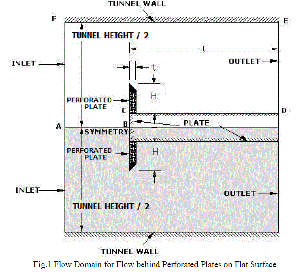
| Numerical investigation was carried out using Computational Fluid Dynamics with the aid of ANSYS Fluent software. Simulation begins with choosing the computational domain, which is the region in space in which the equations of motion are solved. It helps to analyze the problem and to locate the boundaries where the flow conditions are to be applied. Boundaries are to be located where the conditions are known. In the present case, precise conditions were not known and hence the far-field inlet and outlet conditions were applied as 20H on negative side of the origin along x axis and 50H on positive side of the origin along x axis. The two dimensional computational domain chosen is shown in Fig.1. Since the computational domain is symmetrical about the centerline, only half of the domain is considered for simulation to reduce the time of computation and to minimize the memory usage. |
 |
| A. Turbulence Modelling Finite-volume method yields the discretized RANS equations which are solved by Fluent using a cell-centred, segregated approach. Reynolds stresses are the additional unknown variables exhibited by governing equations because of the Reynolds averaging procedure. These Reynolds stresses are to be parameterized for the equation system to be closed and then solved. In the present simulation, the turbulent flow is modelled using Realizable k-ïÃÂÃÂ¥ model. The term "realizable'' means that the model satisfies certain mathematical constraints on the Reynolds stresses, consistent with the physics of turbulent flows. Neither the standard k-ïÃÂÃÂ¥ model nor the RNG k-ïÃÂÃÂ¥ model is realizable. An immediate benefit of the realizable k-ïÃÂÃÂ¥ model is that it more accurately predicts the spreading rate of both planar and round jets. It is also likely to provide superior performance for flows involving rotation, boundary layers under strong adverse pressure gradients, separation, and recirculation. The modelled transport equations for k and ïÃÂÃÂ¥ in the realizable k-ïÃÂÃÂ¥ model are |
 |
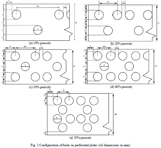
| B. Porous modelling The size and spatial distribution of holes in the normal plate are shown in Fig. 2. Number of the holes decides the level of perforation of individual normal plates. |
 |
| All the computations were 2D with the porous fences modelling as porous regions. In the course of computation cell zone is defined in which the porous media model is applied and the pressure loss in the flow is been fed. Porous media are modelled by the addition of a momentum source term to the standard fluid flow equations. The source term is composed of two parts: a viscous loss term and an inertial loss term |
 |
| where Si is the source term for the ith (x, y, or z) momentum equation, and D and C are prescribed matrices. This momentum sink contributes to the pressure gradient in the porous cell, creating a pressure drop that is proportional to the fluid velocity (or velocity squared) in the cell. To recover the case of simple homogeneous porous media |
 |
| where α is the permeability and C2 is the inertial resistance factor, simply specified D and C as diagonal matrices with 1/ α and C2, respectively, on the diagonal [7] |
| C. Boundary condition At the computational domain inflow (upstream boundaries) Reynolds-averaged velocity components and transported turbulence quantities are specified. A no-slip condition is enforced at the ground. The free stream velocities U∞ are specified at the inlet region which is at a distance of 20 times the fence height in front of the fence [x=0, y varies from 0 to (tunnel height/2)]. For solid boundaries such as plate and tunnel walls, no slip condition is used [u = v = 0]. On the downstream side which is at a distance of 50 times the fence height from the fence, pressure outlet being atmospheric pressure (zero gauge pressure) is specified. |
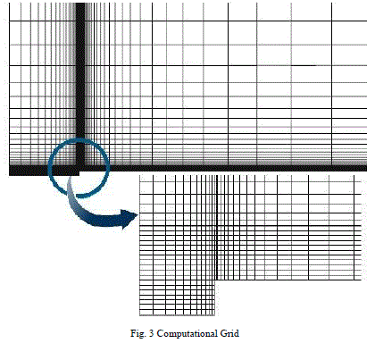
| D. Grid Each cell is a tiny control volume in which discretized versions of the conservation equations are solved. In case of a turbulence model, denser mesh will be considered at the region near the walls than would be needed for a laminar problem. The most important areas obviously are those with the higher gradients, in particular the regions near walls. If it is too coarse, the original mesh may not capture significant effects brought about through steep gradients in the solution. The quality of a CFD solution is highly dependent on the quality of the grid. Therefore, it is necessary that the grid is of high quality before proceeding to the next step. Grids were generated using straight, graded edges. |
 |
| E. Convergence criteria All the computations were continued until the global mass imbalance became smaller than 0.1% of the inlet mass flow rate and until the global specific difference between the RHS and the left-hand side (LHS) of the discretized momentum and turbulence equations became smaller than 0.1% (i.e. ïÿýïÿýïÿýïÿýïÿýïÿý − ïÿýïÿýïÿýïÿýïÿýïÿý / ïÿýïÿýïÿýïÿýïÿýïÿý < 0.001 ) |
III. RESULTS AND DISCUSSIONS |
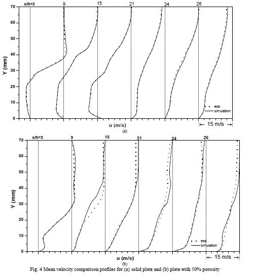
| Mean velocity surveys have been compared for different levels of perforation viz. 0%, 10%, 20%, 30%, 40% and 50% wherein the reference experimental data had been measured using hot-wire anemometer along the centreline of splitter plate at x/h = 3, 9, 15, 21, 24 and 26; covering separation bubble region, reattachment region and some part of redeveloped region. Fig. 4 shows mean velocity profiles of normal solid plate and normal plate with 50% porosity. The numerical simulation predicts well the stable bubble as mentioned in literature. The maxima and minima of the velocity profiles in the region of reverse flow and their fast disappearance in the region of attached flow are well predicted by Realisable k-ε model with maximum variation of 4%. The model indicates higher value of maximum velocity at the edge of the boundary layer which is due the blockage effect of the flow. |
 |
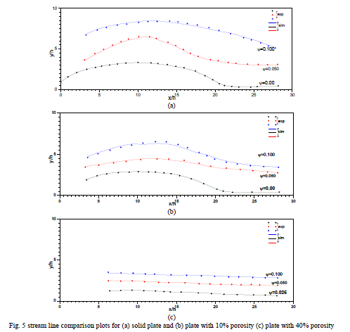
| Stream line plot in Fig.5 compares the experimental data and results of simulation for various levels of perforation. Streamline corresponding to ïÃÂÃâ¢=0 which defines the shape of separated bubble, undergoes drastic changes depending upon the level of perforation level; has been predicted well by the Realizable k-ε model. As inferred from the experimental data, numerical simulation also shows that for the perforation level greater than 30%, the identity of the bubble cannot be traced. |
 |
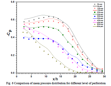
| Fig. 6 shows the mean pressure distribution on the splitter plate for varied degree of perforation of the normal plate obtained from both simulation and experimentation for free stream velocity of 15m/s. The existence of the pressure recovery, depicted by the results of wind tunnel tests, has found to be predicted adequately by computation through the Realizable k-ε model. It can be seen that the behaviour of pressure recovery is same for plates with perforation of 0%, 10%, 20% and 30% wherein the pressure first decreases and then increases. In the case of 40% and 50% porosities, the pressure rise is monotonic which could be attributed to the non-existence of recirculation bubble. The maximum variation of pressure coefficient predicted by simulation is found to be 6% from the literature [1] |
 |
IV. CONCLUSION |
| On a fine grid, “Realizable k-ε closure” from Fluent software has found to give results that are in good qualitative agreement with the observed mean winds. The bubbleâÃâ¬ÃŸs existence and reattachment length for various levels of perforation of the plates is well captured by the numerical simulation. The reattachment length, XR, obtained from the simulation overestimates the results of flow visualisation by a factor of 4% while the original research paper from which the experimental data is taken mentions a maximum possible uncertainty of 5% in location of reattachment length. Outcome of the numerical simulation highlights the reduction in size of recirculation bubble, both in height and length, upto the perforation level of 30% and sweeping away of bubble for higher perforations; as evident by the experimental results. |
References |
|