Canny operator has proved as an optimal edge detector due to due to good localization, detection and only one response to single response. However it has some drawbacks. An improved algorithm has proposed by Gao Lie in which bilateral filtering is used that have better edge preserving and noise removing capabilities. For achieving adaptive thresholding OTSU‟s method is used which automatically calculates the appropriate threshold values for a test image. This improved canny operator performs better than traditional canny operator, lower the probability of detecting the false edges and adaptive in nature. In this paper, we analyse the performance of this improved algorithm .We work on mobile images, containing noise, of different resolutions. The results of experiments show that it performs better for high resolution images but fail to find edges for mobile images of low resolution.
Keywords |
| Canny operator, bilateral filtering, edge detection, OTSU. |
INTRODUCTION |
| Edges are significant local changes of intensity in an image. Edges typically occur on the boundary between two
different regions in an image. So it has fundamental importance in digital image processing. It is basically a method of
segmenting an image into regions of discontinuity. It is a basic tool used in image processing, basically for feature
detection and extraction, which aim to identify points in a digital image where brightness of image changes sharply and
find discontinuities. The purpose of edge detection is significantly reducing the amount of data in an image and
preserves the structural properties for further image processing. [1][2]. Prior classical operators like Robert, Prewitt ,
Sobel etc were used but they didn‟t give satisfactory result as they all are highly sensitive to the noise so detects false
and un sharp edges. |
| In 1986, John F. Canny proposed a new edge detection algorithm; known by this name “Canny edge
detection Algorithm” It is widely considered to be the standard edge detection algorithm in the industry. The aim of
John F. Canny was to find such an algorithm for edge detection provides good detection good localization and minimal
responses. [3] |
| But however it suffers from some drawbacks. Firstly use of Gaussian filter resulted into detecting more
false edges as it smoothened the edges also with noise .Second; operator was not adaptive in nature. Thresholding is
important operation in edge detection. Canny operator use double thresholding concept which uses two threshold
values, high and low. But it is required to set manually and lots of experiments are required to find appropriate values
for an image. |
| To solve above mentioned problems Go Jie has proposed an improved canny algorithm that uses bilateral
filtering instead of Gaussian filter. Bilateral filtering smoothes images while preserving edges, by means of a nonlinear
combination of nearby image values. OTSU‟s method is used for achieving adaptive thresholding. It maximizing the
separability of the resultant classes of gradient magnitude.[4]. However this algorithm performs better for high quality
of images. |
THE TRADITIONAL CANNY OPERATOR [4][5][6] |
| It was proposed by John F. canny in 1986.It is considered as an optimal edge detector. The aim of John F. Canny is to
find such an algorithm for edge detection which full fills following criteria: |
| 1. Good Detection: There should be maximum probability of detecting real edge point and minimum of false edge
points. This results in to the maximized signal to noise ratio. |
| 2. Good Localization: There should be maximum possibility of detected edge closeness to the real edges. |
| 3. Minimal Responses: One real image should result in to only one detected image.[4] |
| A. Canny edge detection algorithm |
| STEP 1: Noise reduction by smoothing with Gaussian Filter. |
| It is well known that whatever we capture from a camera will contain some amount of noise, so there is a probability of
mistaken noise as an edge, therefore noise is required to detect and removed. This is done by smoothing the image by
using Gaussian Filter. Convolution of raw image I i, j is carried out with Gaussian filter G. Assuming the 2-D
Gaussian function as: |
 |
| Where �� is indicates the standard variance of Gaussian function, and it determines the width of the Gaussian filter and
outcome of smoothing. |
| Mathematically, the smooth resultant image is given by |
| F (i, j) = G * I( i, j) |
| STEP 2: Finding gradients |
| In this step we detect the edges where the change in greyscale intensity is maximum. Required areas are determined
with the help of gradient of images. Sobel operator is used to determine the gradient at each pixel of smoothened
image. Sobel operators in i and j directions are given as |
 |
| These sobel masks are convolved with smoothed image and giving gradients in i and j directions. |
 |
| Therefore edge strength or magnitude of gradient of a pixel is given by |
 |
| The direction of gradient is given by |
 |
| Gi And Gj are the gradients in the i- and j-directions respectively. |
| STEP 3: Non maximum suppressions: |
| Non maximum suppression is carried out to preserves all local maxima in the gradient image, and deleting everything
else this results in thin edges. For a pixel M (i, j): |
| Firstly round the gradient direction �� nearest45°,then compare the gradient magnitude of the pixels in positive and
negative gradient directions i.e. If gradient direction is east then compare with gradient of the pixels in east and
west directions say E (i, j) and W (i, j) respectively |
| If the edge strength of pixel M (i, j) is largest than that of E (i, j) and W (i, j), then preserve the value of gradient
and mark M (i, j) as edge pixel, if not then suppress or remove. |
| STEP 4: Hysteresis thresholding: |
| The output of non-maxima suppression still contains the local maxima created by noise. Instead choosing a single
threshold, for avoiding the problem of streaking two thresholds 349; are used. For a pixel M (i, j) having
gradient magnitude G following conditions exists to detect pixel as edge: |
| • If G < tlow than discard the edge. |
| • If G > than thigh keep the edge. |
| • If tlow< G < and thigh and any of its neighbors in a 3 ×3 region around it have gradient magnitudes greater
than thigh keep the edge. |
| If none of pixel (x, y)‟s neighbors have high gradient magnitudes but at least one falls between tlow and, thigh
search the 5 × 5 region to see if any of these pixels have a magnitude greater than thigh. If so, keep the edge. |
| • Else, discard the edge. |
| B. Demerits of traditional canny operator |
| The traditional canny operator is suffered from following negative points: |
| 1. Use of Gaussian filtering, smoothes the important edges while removing the noise. This weakened the edges and
increases false edges detection. |
| 2. Double thresholding is used which require to set high and low threshold values manually,
To get appropriate threshold values for an image several experiments are required. |
THE IMPROVED CANNY OPERATOR [7] |
| It has proposed by Gao Jie and Liu Ning .They use bilateral filter instead of Gaussian filter and use OTSU‟s method for
thresholding. |
| A. Bilateral filtering [8] |
| Instead of Gaussian filter bilateral filtering is used to reduce the probability of false edges detection. |
| 1). Introduction: The conventional canny operator suffers from the problem of detecting false edges and smoothes
edges with noise. In 1988, C.Tomasi and R.Manduchi proposed bilateral filtering. A bilateral filter is used for edge
preservation and noise reduction for digital images. For an image, it replaces the intensity value of a pixel by weighted
average of intensity values of the nearby pixels. |
| Gaussian low-pass filtering computes a weighted average of pixel values in the neighbourhood, in which,
the weights decrease with distance from the neighbourhood centre.
Although formal and quantitative explanations of this weight fall-off can be given the intuitions that images typically
vary slowly over space, so near pixels are likely to have similar values, and it is therefore appropriate to average them
together. The noise values that corrupt these nearby pixels are mutually less correlated than the signal values, so noise
is averaged away while signal is preserved. |
| 2). Mathematical Analysis of bilateral Filtering: For image f(a), on applying low-pass filter, the filtered image is given
by |
 |
| Where c( , x) denotes the geometric closeness between the neighbourhood centre „a‟ and a nearby point . Filter
output is the integral of the input signal along having adaptive weight functions which are obtained from the average of
the pixels information of the nearby region. These weights are called filter kernels. For spacial domain, it is denoted by
c(ξ), where ξ is the offset vector which measures position in the local neighbourhood of a and represents the closeness
between the point a and ξ .Where |
 |
| is the normalizing factor to preserve the dc components of the low pass signals. |
| A filtering window is created around a, which depends on the value of ξ. If the point lie within
the window, c(ξ) has a considerable value so the integral can be taken into account. But if the points lie beyond this
region, c(ξ) value diminishes and integral don‟t have ny value. |
| After applying Range filtering, for an input image f(a) the filtered image is given by |
 |
| Where indicates the photometric �� f(), ��(��) similarity between the center pixel x and its neighborhood point. |
| Where |
 |
| is normalizing factor that preserves the dc components of the low pass signals. |
| Contrary to what occurs with the geometric closeness, the photometric similarity is determined by the difference f ()
−f (a). On combining domain and range filtering, bilateral filtering is given by following |
 |
| This combination of spatial and domain filtering is called as bilateral filtering. Its plus factor is that that it replaces the
pixel value at a, with an average of similar and nearby pixel values. Bilateral filtering performs as a standard domain filter for smooth regions. As in smooth regions, neighbourhood pixels values are same and approximating a constant. In
sharp region, the filter replaces the bright pixel at the centre by an average of surrounding bright pixels, and ignores the
dark pixels. Conversely, when the filter is cantered on a dark pixel, the bright pixels are ignored instead. Thus, the
bilateral filtering does not only filter the noise, but also preserve the edges of image, which is practical method that can
be put into practice to a great extent. |
| B. OTSU’s method, adaptive thresholding [9] |
| In order to make canny operator adaptive, OTSU‟s thresholding is used n new algorithm. |
| 1). Introduction: Otsu's method is based on image histogram process. It performs histogram shape-based image
thresholding automatically. The algorithm assumes that the thresholding image is divided into two classes of pixels
(foreground and background), then it calculates the optimum threshold which separates these two classes such that they
have minimal intra-class variance. |
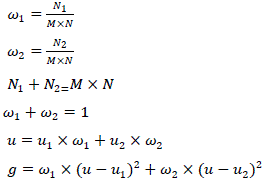
| 2). Mathematical Analysis :For an M ×N image I (x, y), the segmented threshold of foreground and background denotes
as T, the rate of foreground is 1, its average value is 1; the rate of the background is 2 and the average value is 2 ,
the mean of the image is u , the variance of the inter-class is g. Then we can get the following formulas: |
 |
| From the above formulation, following formula can be obtained: |
 |
| Finally, applying traversed approach to obtain the threshold which makes g maximum, and then T is the optimal
threshold. As a sequence, we consider T as the high threshold, and the low threshold can be got as: |
 |
STEPS OF IMPROVED ALGORITHM |
| 1) Smooth the input image by using bilateral filtering: Bilateral filter sharply detect and preserve the edges. The
probability of false edges is reduced. |
| 2) Find the gradient magnitude and direction: Same procedure as in traditional canny operators. |
| 3) Perform non maximum suppression: Same procedure as in traditional canny operator. |
| 4) Adaptively determine threshold using OTSU’s method and find the connected edges: OTSU‟s method
determine two thresholds T1 (high threshold) and T2 (low threshold) then mark a point say P (i, j) as candidate pixel
and find its gradient say G (i, j). Two conditions are there: |
| i) If G (i, j) > T1 then P (i, j) is absolutely an edge point. |
| ii) If G (i, j) < T2 then P (i, j) is absolutely not an edge point. |
RESULTS AND ANALYSIS |
| The new algorithm is implemented using MTLAB tool. In this paper we perform on different megapixels of images and
analysis the performance of this new algorithm. Following results are obtained: |
| A. Compare with traditional canny operator: |
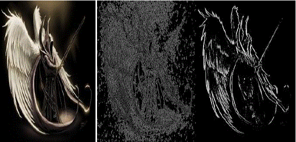
| As we can see in the figure (b) that canny operator gives false edges as it consider noise as edges while this new
proposed algorithm gives fine edges as shown in figure(c). |
| B. Performance analysis with different resolution of real time image taken from mobile |
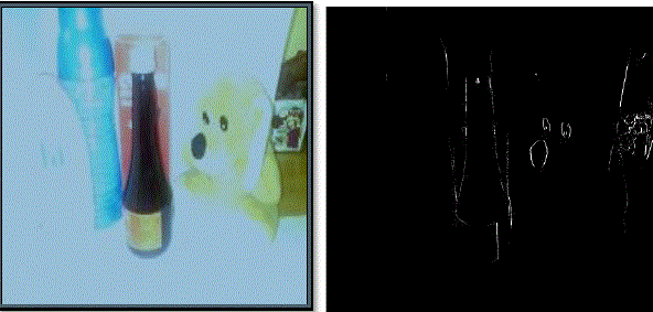
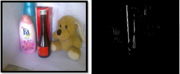
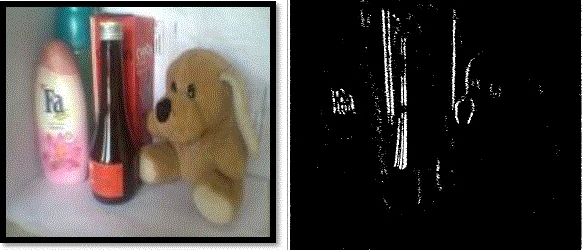
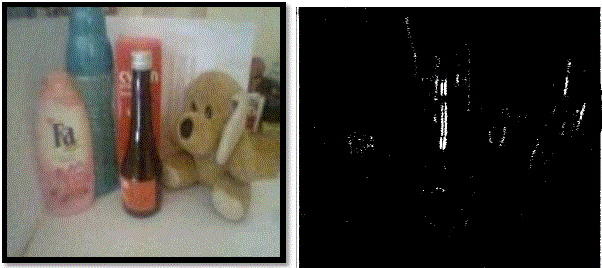
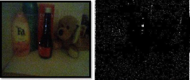
| On implementing improved canny operator on Matlab, using different resolution of mobile images, above results are
obtained. We can see that, for a high mega pixel image taken from mobile like 5MP this operator finds sharp and clear
edges as shown in fig. 2, as the resolution of mobile decreases the edge detection ability of detector decreases and
hence results into thick and blurred edges. Fig.4 having test image of 1.2 MP, results into some blurred and thick edges.
Fig.5 shows test image of 0.5 MP resolutions, operator gives very blurred edges Fig 6 shows lowest resolution image of
0.1 MP, operator fails to detect the edges of this image. |
CONCLUSION |
| Edge detection is an important segmentation process carried out in digital image processing. Canny edge algorithm is
considered as optimal edge detection technique but it responds to false image in noisy environment and is not adaptive
in nature. For a high resolution image , this new proposed algorithm, using bilateral filtering and adaptive OTSU‟s
thresholding, performs better than traditional canny operator .I have worked on this new improved canny operator on
different resolution mobile images using MATLAB. On implementing this algorithm on high resolution of mobile
image like 5 MP, it has been seen that it results into fine sharp edges. And As we can seen from the above figures that
this proposed algorithm results into thick and some false edges as resolution of mobile camera goes down. For lower
resolution image like 0.1 MP it is unable to find the edges. It has also been noticed that for light colour objects it is
unable to find edges. So further work can be done in future to overcome these deficiencies, of this new operator. |
ACKNOWLEDGEMENT |
| I would like to express my deepest appreciation to all those who provided me the possibility to complete this research
paper. A special gratitude we give to our guide Er. Mukesh Kumar, Department of Electronics and Communication
Engineering SSET SHIATS India, whose contribution in stimulating suggestions, encouragement, and guidance helped
me to coordinate our research work and achieve the goal successfully. |
| Furthermore I would also like to acknowledge with much appreciation the crucial role of our HOD, Prof. A.K.
Jaiswal, Department of Electronics and Communication Engineering SSET SHIATS India, for his devoted
encouragement towards the completion of research paper. |
Figures at a glance |
 |
 |
 |
| Figure 1 |
Figure 2 |
Figure 3 |
 |
 |
 |
| Figure 4 |
Figure 5 |
Figure 6 |
|
References |
- Jonathan M. Black ledge, „Digital Image Processing Mathematical and Computational Methods‟, Coll House, Watergate, Chic ester, West Sussex, PO20 3QL, England, 2005.
- R .Gonzalez and R. Woods, ‘ Digit al Image Processing‟, Addison Wesley, pp 414 – 428, 1992.
- J. Canny, “A computational approach to edge detection,” IEEE Trans. Pattern Analysis and Machine Intelligence, Vol. 8 No. 6, pp. 679-698, 1986.
- CANNY EDGE DETECTION http://homepage.cs.uiowa.edu/~cwyman/classes/spring08-22C251/homework/canny.pdf
- Canny Edge Detection, March 23, 2009 http://www.cse.iitd.ernet.in/~pkalra/csl783/canny.pdf.
- S. Sridhar, „Digital Image Processing‟, Oxford University Press, 2011.
- Gao Jie, Liu Ning, „An improved adaptive threshold canny edge detection algorithm‟, IEEE Transactions, International Conference on Computer Science and Electronics Engineering, Vol. 1, pp.164-168, 2012, 2012.
- C.Tomasi, R. Manduch, „Bilateral Filtering for Gray and Color Images‟, Proceedings of the 1998 IEEE International Conferences on Computer Vsion.Bombay, India, Vol.5, pp. 839-846, 1998.
- Nobuyuki Otsu, „A threshold selection method from gray-level histogram‟ [J]. IEEE Transactions on System, Man, Cybernetics, Vol. 9, pp. 62-66, 1979.
|