The Usefulness of Implicit Regression in Model Quality

Implicit Regression

Implicit Regression is useful in measuring the constant nature of a measured variable [1]; it helps detect bivariate and multivariate random error; it is sensitive to incorrect modeling; and can handle co-dependent relationships more readily than standard non-linear regression [2,3].

Implicit Regression [4,5] using ordinary least squares to determine parameter estimates for models of the form

Where is a fixed function with well-defined constant coefficients and is defined in terms of the unknown coefficients

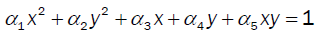
The only restriction is uniqueness of the terms; that is, given the terms of interest where N is the number of terms to be considered, then terms contained in the function may not be contained in the function . Common terms include unity (a column vector of 1), individual measures, higher order terms and interaction terms; that is

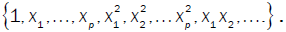
There are two types of resulting analysis: Non-response Analysis and Rotational Analysis. Non-response analysis is where whereas Rotational Analysis allows for each term other than unity to be taken as the response variable in turn.

The first use is the same in both standard regression and the non-response model defined under Implicit Regression which is the explanatory power otherwise referred to as the coefficient of determination, R².

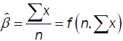
In univariate, the explanatory power is a function of the sample size, the sum of the data and the sum of squares and is given by

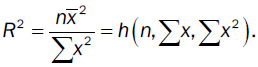
This is the percent variance explained by the mean. This is a measure of the constant nature of a “variable”. Variable here is placed in quotations because as R² →1, the smaller the variance and the measure is less variant and may be consider a constant, relatively speaking.

The measure the explanatory power is the same using standard regression and non-response analysis with analytical forms.

respectively. The first of which minimize the variance and the solution is

The second met 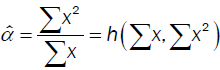hod minimizes the coefficient of variation with solution

Notice that the explanatory power is the ratio of these two point estimates:

In bivariate, there are three rotations in simple linear relationships:

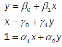
These models are such that the parameter estimates are functions of the summary statistics: the sample size, the sums, the sums of the products and the sum of the squares:

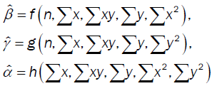
where the solutions to the non-response model does not depend on the sample size, but rather the base variance (Wooten R. D., 2016). Like turning the end of a kaleidoscope, these rotational views give more insight to the relationship that exist between the measures including the possibility of a co-dependent relationship that does not depend on the sample size.

Consider the following simulation: let x ~ U(10,100) and y = x^a, and the observed value (x_i,y_i) contain random error 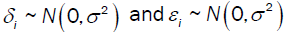, respectively. That is, bivariate error:

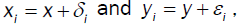
Consider the following four cases:

Consider the three rotations with σ = 2,5,10 in the four outlined cases, illustrated on the next page. Standard regression is shown in red and green; and implicit regression is shown in green. The larger the variance, the larger the pin wheel effect; however, when the relationship is non-linear, the effect is more pronounced. That is, comparing the graphics when there is small variance in a simple linear relationship, then the three rotations converge. However, when there is large variance or a non-linear relationship, the graphics show a pin-wheel effect.

Implicit Regression enables the researcher to detect bivariate random error and model non-linear co-dependent relationships in multivariate analysis (Figure 1).

Figure 1: Fitting a linear model to linear and non-linear relationships. The four cases are illustrated by increasing deviations

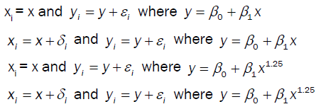
First consider the bivariate example of a circle with unit deviation and sinusoidal frequency; that is, the equation (x-100)2+(y - 100)2=6.25, that both accelerate and decelarate based on time. The data was simulated using the following algorithm over 10 periods:

The resulting data creates the random pattern shown in Figure 2

Figure 2. Scatter plot of simulated data as matched pairs (x_i,y_i ).

Where,

The resulting solution shown in green, (Figure 3), is representative of the underlying relationship shown in red and the observed data in blue. Implicit regression also detected that the term xy was insignificant.

Figure 3. Scatter plot of simulated data (x_i,y_i ) in blue, the solutions to the developed model in green, and the underlying variables. (x,y)

As the assumption of independence is not required, Implicit Regression does not have the same measure of explanatory power and is subject to the tractability of the individual variables. There are three measures of error in modeling between the following measures: the data , the central tendencies and the resulting surface obtained by the developed model 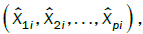The total errors are 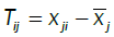and the errors explained by the model are 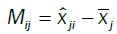and the residual errors are

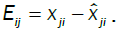
In Standard Regression, under the assumption of independence and limitations placed on terms, the Pythagorean Theorem holds for the measured response:

SST = SSM + SSE.

That is, when given 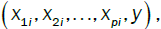where the model is of the form and the error terms are only taken for this single variable, does this relationship hold true.

Using Implicit Regression, we can consider all variables individually or in combinations using the extended formula for law of cosines which is given by

The angle is the degree of separation between M and E in the vector space created by M, E and T. The degree of separation can be measured one variable at a time with for the selected variable x_j with

Moreover, you can assess the degree of separation between subsets of variables or all the variables as illustrated in the vector space below.

The closer the degree of separation is to 90°, the stronger the independent relationship between the three measured errors.

References

1. Wooten RD, et al. Implicit regression: Detecting constants and inverse relationships with bivariate random error. Cornell University Library, 2015.
2. Wooten RD. Statistical analysis of the relationship between wind speed, pressure and temperature. Journal of Applied Sciences. 2011.
3. Wooten RD and D'AndreaJ. Modeling hurricanes using principle component analysis in conjunction with non-response analysis. Cornell University Library. 2016.
4. Wooten RD. An introduction to implicit regression: Extending standard regression to rotational analysis and non-response analysis. Cornell University Library. 2016.
5. Wooten RD. Lattice designs in standard and simple implicit multi-linear regression. Cornell University Library. 2016.